 Redbooth, makers of project management and collaboration software, announced a new Apple TV app today that brings their service directly to Apple TV. We mostly think of Apple TV as a consumer device, designed to give us access to entertainment and games or to project the contents of one of our Apple devices onto a bigger screen. That changed to some extent last year when Apple announced… Read More
Aug
18
2016
18
2016
--
Redbooth adds Apple TV app to bring project management to big screen
Aug
18
2016
18
2016
--
Atlassian’s HipChat gets group video chats
 In Atlassian‘s view, video is the next battlefield in the enterprise chat wars (a war it is mostly fighting with Slack, it seems). Its HipChat group messaging app launched one-on-one video chats back in 2014, but today, it is pushing this further by launching group video chats, as well.
To enable this, Atlassian built a new video platform based on its acquisition of BlueJimp and that… Read More
Aug
17
2016
17
2016
--
Cisco confirms it will cut up to 5,500 jobs, or 7% of its global workforce
 We caught wind earlier this week that Cisco was planning a major cost-cutting operation to reduce its costs by around 15% throughout the month. It looks like the first stage of that is a round of cut jobs, with Cisco announcing as part of its earnings report that it will cut up to 5,500 jobs, or 7% of its workforce. The move isn’t unexpected as Cisco works to transition to a new era where… Read More
Aug
17
2016
17
2016
--
Netlify, a service for quickly rolling out static websites, raises $2.1M
 Mathias Biilmann — a former CTO of a firm that built websites for small businesses — says developers have gotten so used to using Github as a central workflow, they expect the entire rest of the developer experience to work the same way. “The way that a front-end developer would work would be to go into a server and change how things were structured, but then Git came in… Read More
Aug
17
2016
17
2016
--
Improve TokuDB/PerconaFT fragmented data file performance
In this blog post, we’ll discuss how to improve TokuDB and PerconaFT fragmented data file performance.
Through our internal benchmarking and some user reports, we have found that with long term heavy write use TokuDB/PerconaFT performance can degrade significantly on large data files. Using smaller node sizes makes the problem (which is one of our performance tuning recommendations when you have faster storage). The problem manifests as low CPU utilization, a drop in overall TPS and high client response times during prolonged checkpointing.
This post explains a little about how we structure PerconaFT dictionary files and where the current implementation breaks down. Hopefully, it explains the nature of the issue, and how our solution helps addresses it. It also provides some contrived benchmarks that prove the solution.
PerconaFT map file disk format
NOTE. This post uses the terms index, data file, and dictionary are somewhat interchangeable. We will use the PerconaFT term “dictionary” to refer specifically to a PerconaFT key/value data file.
PerconaFT stores every dictionary in its own data file on disk. TokuDB stores each index in a PerconaFT dictionary, plus one additional dictionary per table for some metadata. For example, if you have one TokuDB table with two secondary indices, you would have four data files or dictionaries: one small metadata dictionary for the table, one dictionary for the primary key/index, and one for each secondary index.

Each dictionary file has three major parts:
- Two headers (yes, two) made up of various bits of metadata, file versions, a checkpoint logical sequence number (CLSN), the offset of this headers block translation table, etc…
- Two (yes, two, one per header) block translation tables (BTT) that maps block numbers (BNs) to the physical offsets and sizes of the data blocks within the file.
- Data blocks and holes (unused space). Unlike InnoDB, PerconaFT data blocks (nodes) are variable sizes and can be any size from a minimum of a few bytes for an empty internal node all the way up to the block size defined when the tree created (4MB by default if we don’t use compression) and anywhere in between, depending on the amount of data within that node.
Each dictionary file contains two versions of the header stored on disk, and only one is valid at any given point in time. Since we fix the size of the header structure, we always know their locations. The first at offset zero, the other is immediately after the first. The header that is currently valid is the header with the later/larger CLSN.
We write the header and the BTT to disk during a checkpoint or when a dictionary is closed (the only time we do so). The header overwrites the older header (the one with the older CLSN) on disk. From that moment onward, the disk space used by the previous version of the dictionary (the whole thing, not just the header) that is not also used by the latest version, is considered immediately free.
There is much more magic to how the PerconaFT does checkpoint and consistency, but that is really out of the scope of this post. Maybe a later post that addresses the sharp checkpoint of the PerconaFT can dive into this.
The block allocator
The block allocator is the algorithm and container that manages the list of known used blocks and unused holes within an open dictionary file. When a node gets written, it is the responsibility of the block allocator to find a suitable location in the file for the nodes data. It is always placed into a new block, never overwrites an existing block (except for reclaimed block space from blocks that are removed or moved and recorded during the last checkpoint). Conversely, when a node gets destroyed it is the responsibility of the block allocator to release that used space and create a hole out of the old block. That hole also must be merged with any other holes that are adjacent to it to have a record of just one large hole rather than a series of consecutive smaller holes.
Fragmentation and large files
The current implementation of the PerconaFT block allocator maintains a simple array of used blocks in memory for each open dictionary. The used blocks are ordered ascending by their offset in the file. The holes between the blocks are calculated by knowing the offset and size of the two bounding blocks. For example, one can calculate the hole offset and size between two adjacent blocks as: b[n].offset + b[n].size and b[n+1].offset – (b[n].offset + b[n].size), respectively.

To find a suitable hole to place node data, the current block allocator starts at the first block in the array. It iterates through the blocks looking for a hole between blocks that is large enough to hold the nodes data. Once we find a hole, we cut the space needed for the node out of the hole and the remainder is left as a hole for another block to possibly use later. Note : There is overhead to force alignment to 512 offsets for direct i/o regardless if direct i/o is used or not.
Note. Forcing alignment to 512 offsets for direct I/O has overhead, regardless if direct I/O is used or not.
This linear search severely degrades the PerconaFT performance for very large and fragmented dictionary files. We have some solid evidence from the field that this does occur. We can see it via various profiling tools as a lot of time spent within block_allocator_strategy::first_fit. It is also quite easy to create a case by using very small node (block) sizes and small fanouts (forces the existence of more nodes, and thus more small holes). This fragmentation can and does cause all sorts of side effects as the search operation locks the entire structure within memory. It blocks nodes from translating their node/block IDs into file locations.
Let’s fix it…
In this block storage paradigm, fragmentation is inevitable. We can try to dance around and propose different ways to prevent fragmentation (at the expense of higher CPU costs, online/offline operations, etc…). Or, we can look at the way the block allocator works and try to make it more efficient. Attacking the latter of the two options is a better strategy (not to say we aren’t still actively looking into the former).
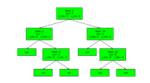
Tree-based “Max Hole Size” (MHS) lookup
The linear search block allocator has no idea where bigger and smaller holes might be located within the set (a core limitation). It must use brute force to find a hole big enough for the data it needs to store. To address this, we implemented a new in-memory, tree-based algorithm (red-black tree). This replaces the current in-memory linear array and integrates the hole size search into the tree structure itself.
In this new block allocator implementation, we store the set of known in-use blocks within the node structure of a binary tree instead of a linear array. We order the tree by the file offset of the blocks. We then added a little extra data to each node of this new tree structure. This data tells us the maximum hole we can expect to find in each child subtree. So now when searching for a hole, we can quickly drill down the tree to find an available hole of the correct size without needing to perform a fully linear scan. The trade off is that merging holes together and updating the parental max hole sizes is slightly more intricate and time-consuming than in a linear structure. The huge improvement in search efficiency makes this extra overhead pure noise.

We can see in this overly simplified diagram, we have five blocks:
- offset 0 : 1 byte
- offset 3 : 2 bytes
- offset 6 : 3 bytes
- offset 10 : 5 bytes
- offset 20 : 8 bytes
We can calculate four holes in between those blocks:
- offset 1 : 2 bytes
- offset 5 : 1 byte
- offset 9 : 1 byte
- offset 15 : 5 bytes
We see that the search for a 4-byte hole traverses down the right side of the tree. It discovers a hole at offset 15. This hole is a big enough for our 4 bytes. It does this without needing to visit the nodes at offsets 0 and 3. For you algorithmic folks out there, we have gone from an O(n) to O(log n) search. This is tremendously more efficient when we get into severe fragmentation states. A side effect is that we tend to allocate blocks from holes closer to the needed size rather than from the first one big enough to fit. The small hole fragmentation issue may actually increase over time, but that has yet to be seen in our testing.
Benchmarks
As our CTO Vadim Tkachenko asserts, there are “Lies, Damned Lies and Benchmarks.” We won’t convince you using some pseudo-real-world benchmark that uses sleight of hand. We’re going to show a simple test case where we thought, “What is the worst possible scenario that I can come up with in a small-ish benchmark to show the differences?”.
That scenario is actually pretty simple. We shape the tree to have as many nodes as possible, and intentionally use settings that reduce concurrency. We will use a standard sysbench OLTP test, and run it for about three hours after the prepare stage has completed:
- Hardware:
- Intel i7, 4 core hyperthread (8 virtual cores) @ 2.8 GHz
- 16 GB of memory
- Samsung 850 Pro SSD
- Sysbench OLTP:
- 1 table of 160M rows or about 30GB of primary key data and 4GB secondary key data
- 24 threads
- We started each test server instance with no data. Then we ran the sysbench prepare, then the sysbench run with no shutdown in between the prepare and run.
- prepare command : /data/percona/sysbench/sysbench/sysbench –test=/data/percona/sysbench/sysbench/tests/db/parallel_prepare.lua –mysql-table-engine=tokudb –oltp-tables-count=1 –oltp-table-size=160000000 –mysql-socket=$(PWD)/var/mysql.sock –mysql-user=root –num_threads=1 run
- run command : /data/percona/sysbench/sysbench/sysbench –test=/data/percona/sysbench/sysbench/tests/db/oltp.lua –mysql-table-engine=tokudb –oltp-tables-count=1 –oltp-table-size=160000000 –rand-init=on –rand-type=uniform –num_threads=24 –report-interval=30 –max-requests=0 –max-time=10800 –percentile=99 –mysql-socket=$(PWD)/var/mysql.sock –mysql-user=root run
- mysqld/TokuDB configuration
- innodb_buffer_pool_size=5242880
- tokudb_directio=on
- tokudb_empty_scan=disabled
- tokudb_commit_sync=off
- tokudb_cache_size=8G
- tokudb_checkpointing_period=300
- tokudb_checkpoint_pool_threads=1
- tokudb_enable_partial_eviction=off
- tokudb_fsync_log_period=1000
- tokudb_fanout=8
- tokudb_block_size=8K
- tokudb_read_block_size=1K
- tokudb_row_format=tokudb_uncompressed
- tokudb_cleaner_period=1
- tokudb_cleaner_iterations=10000


So as you can see: amazing results, right? Sustained throughput, immensely better response time and better utilization of available CPU resources. Of course, this is all fake with a tree shape that no sane user would implement. It illustrates what happens when the linear list contains small holes: exactly what we set out to fix!
Closing
Look for this improvement to appear in Percona Server 5.6.32-78.0 and 5.7.14-7. It’s a good one for you if you have huge TokuDB data files with lots and lots of nodes.
Credits!
Throughout this post, I referred to “we” numerous times. That “we” encompasses a great many people that have looked into this in the past and implemented the current solution. Some are current and former Percona and Tokutek employees that you may already know by name. Some are newer at Percona. I got to take their work and research, incorporate it into the current codebase, test and benchmark it, and report it here for all to see. Many thanks go out to Jun Yuan, Leif Walsh, John Esmet, Rich Prohaska, Bradley Kuszmaul, Alexey Stroganov, Laurynas Biveinis, Vlad Lesin, Christian Rober and others for all of the effort in diagnosing this issue, inventing a solution, and testing and reviewing this change to the PerconaFT library.
Aug
17
2016
17
2016
--
How Apache Spark makes your slow MySQL queries 10x faster (or more)

 In this blog post, we’ll discuss how to improve the performance of slow MySQL queries using Apache Spark.
Introduction
In my previous blog post, I wrote about using Apache Spark with MySQL for data analysis and showed how to transform and analyze a large volume of data (text files) with Apache Spark. Vadim also performed a benchmark comparing performance of MySQL and Spark with Parquet columnar format (using Air traffic performance data). That works great, but what if we don’t want to move our data from MySQL to another storage (i.e., columnar format), and instead want to use “ad hock” queries on top of an existing MySQL server? Apache Spark can help here as well.
TL;DR version:
Using Apache Spark on top of the existing MySQL server(s) (without the need to export or even stream data to Spark or Hadoop), we can increase query performance more than ten times. Using multiple MySQL servers (replication or Percona XtraDB Cluster) gives us an additional performance increase for some queries. You can also use the Spark cache function to cache the whole MySQL query results table.
The idea is simple: Spark can read MySQL data via JDBC and can also execute SQL queries, so we can connect it directly to MySQL and run the queries. Why is this faster? For long running (i.e., reporting or BI) queries, it can be much faster as Spark is a massively parallel system. MySQL can only use one CPU core per query, whereas Spark can use all cores on all cluster nodes. In my examples below, MySQL queries are executed inside Spark and run 5-10 times faster (on top of the same MySQL data).
In addition, Spark can add “cluster” level parallelism. In the case of MySQL replication or Percona XtraDB Cluster, Spark can split the query into a set of smaller queries (in the case of a partitioned table it will run one query per each partition for example) and run those in parallel across multiple slave servers of multiple Percona XtraDB Cluster nodes. Finally, it will use map/reduce the type of processing to aggregate the results.
I’ve used the same “Airlines On-Time Performance” database as in previous posts. Vadim created some scripts to download data and upload it to MySQL. You can find the scripts here: https://github.com/Percona-Lab/ontime-airline-performance. I’ve also used Apache Spark 2.0, which was released July 26, 2016.
Apache Spark Setup
Starting Apache Spark in standalone mode is easy. To recap:
- Download the Apache Spark 2.0 and place it somewhere.
- Start master
- Start slave (worker) and attach it to the master
- Start the app (in this case spark-shell or spark-sql)
Example:
root@thor:~/spark# ./sbin/start-master.sh
less ../logs/spark-root-org.apache.spark.deploy.master.Master-1-thor.out
15/08/25 11:21:21 INFO Master: Starting Spark master at spark://thor:7077
15/08/25 11:21:21 INFO Utils: Successfully started service 'MasterUI' on port 8080.
15/08/25 11:21:21 INFO MasterWebUI: Started MasterWebUI at http://10.60.23.188:8080
root@thor:~/spark# ./sbin/start-slave.sh spark://thor:7077
To connect to Spark we can use spark-shell (Scala), pyspark (Python) or spark-sql. Since spark-sql is similar to MySQL cli, using it would be the easiest option (even “show tables” works). I also wanted to work with Scala in interactive mode so I’ve used spark-shell as well. In all the examples I’m using the same SQL query in MySQL and Spark, so working with Spark is not that different.
To work with MySQL server in Spark we need Connector/J for MySQL. Download the package and copy the mysql-connector-java-5.1.39-bin.jar to the spark directory, then add the class path to the conf/spark-defaults.conf:
spark.driver.extraClassPath = /usr/local/spark/mysql-connector-java-5.1.39-bin.jar
spark.executor.extraClassPath = /usr/local/spark/mysql-connector-java-5.1.39-bin.jar
Running MySQL queries via Apache Spark
For this test I was using one physical server with 12 CPU cores (older Intel(R) Xeon(R) CPU L5639 @ 2.13GHz) and 48G of RAM, SSD disks. I’ve installed MySQL and started spark master and spark slave on the same box.
Now we are ready to run MySQL queries inside Spark. First, start the shell (from the Spark directory, /usr/local/spark in my case):
$ ./bin/spark-shell --driver-memory 4G --master spark://server1:7077
Then we will need to connect to MySQL from spark and register the temporary view:
val jdbcDF = spark.read.format("jdbc").options(
  Map("url" ->  "jdbc:mysql://localhost:3306/ontime?user=root&password=",
  "dbtable" -> "ontime.ontime_part",
  "fetchSize" -> "10000",
  "partitionColumn" -> "yeard", "lowerBound" -> "1988", "upperBound" -> "2016", "numPartitions" -> "28"
  )).load()
jdbcDF.createOrReplaceTempView("ontime")
So we have created a “datasource” for Spark (or in other words, a “link” from Spark to MySQL). The Spark table name is “ontime” (linked to MySQL ontime.ontime_part table) and we can run SQL queries in Spark, which in turn parse it and translate it in MySQL queries.
“partitionColumn” is very important here. It tells Spark to run multiple queries in parallel, one query per each partition.
Now we can run the query:
val sqlDF = sql("select min(year), max(year) as max_year, Carrier, count(*) as cnt, sum(if(ArrDelayMinutes>30, 1, 0)) as flights_delayed, round(sum(if(ArrDelayMinutes>30, 1, 0))/count(*),2) as rate FROM ontime WHERE DayOfWeek not in (6,7) and OriginState not in ('AK', 'HI', 'PR', 'VI') and DestState not in ('AK', 'HI', 'PR', 'VI') and (origin = 'RDU' or dest = 'RDU') GROUP by carrier HAVING cnt > 100000 and max_year > '1990' ORDER by rate DESC, cnt desc LIMIT  10")
sqlDF.show()
MySQL Query Example
Let’s go back to MySQL for a second and look at the query example. I’ve chosen the following query (from my older blog post):
select min(year), max(year) as max_year, Carrier, count(*) as cnt,
sum(if(ArrDelayMinutes>30, 1, 0)) as flights_delayed,
round(sum(if(ArrDelayMinutes>30, 1, 0))/count(*),2) as rate
FROM ontime
WHERE
DayOfWeek not in (6,7)
and OriginState not in ('AK', 'HI', 'PR', 'VI')
and DestState not in ('AK', 'HI', 'PR', 'VI')
GROUP by carrier HAVING cnt > 100000 and max_year > '1990'
ORDER by rate DESC, cnt desc
LIMIT  10
The query will find the total number of delayed flights per each airline. In addition, the query will calculate the smart “ontime” rating, taking into consideration the number of flights (we do not want to compare smaller air carriers with the large ones, and we want to exclude the older airlines who are not in business anymore).
The main reason I’ve chosen this query is that it is hard to optimize it in MySQL. All conditions in the “where” clause will only filter out ~70% of rows. I’ve done a basic calculation:
mysql> select count(*) FROM ontime WHERE DayOfWeek not in (6,7) and OriginState not in ('AK', 'HI', 'PR', 'VI') and DestState not in ('AK', 'HI', 'PR', 'VI');
+-----------+
| count(*)  |
+-----------+
| 108776741 |
+-----------+
mysql> select count(*) FROM ontime;
+-----------+
| count(*)  |
+-----------+
| 152657276 |
+-----------+
mysql> select round((108776741/152657276)*100, 2);
+-------------------------------------+
| round((108776741/152657276)*100, 2) |
+-------------------------------------+
|                               71.26 |
+-------------------------------------+
Table structure:
CREATE TABLE `ontime_part` (
  `YearD` int(11) NOT NULL,
  `Quarter` tinyint(4) DEFAULT NULL,
  `MonthD` tinyint(4) DEFAULT NULL,
  `DayofMonth` tinyint(4) DEFAULT NULL,
  `DayOfWeek` tinyint(4) DEFAULT NULL,
  `FlightDate` date DEFAULT NULL,
  `UniqueCarrier` char(7) DEFAULT NULL,
  `AirlineID` int(11) DEFAULT NULL,
  `Carrier` char(2) DEFAULT NULL,
  `TailNum` varchar(50) DEFAULT NULL,
...
  `id` int(11) NOT NULL AUTO_INCREMENT,
  PRIMARY KEY (`id`,`YearD`),
  KEY `covered` (`DayOfWeek`,`OriginState`,`DestState`,`Carrier`,`YearD`,`ArrDelayMinutes`)
) ENGINE=InnoDB AUTO_INCREMENT=162668935 DEFAULT CHARSET=latin1
/*!50100 PARTITION BY RANGE (YearD)
(PARTITION p1987 VALUES LESS THAN (1988) ENGINE = InnoDB,
 PARTITION p1988 VALUES LESS THAN (1989) ENGINE = InnoDB,
 PARTITION p1989 VALUES LESS THAN (1990) ENGINE = InnoDB,
 PARTITION p1990 VALUES LESS THAN (1991) ENGINE = InnoDB,
 PARTITION p1991 VALUES LESS THAN (1992) ENGINE = InnoDB,
 PARTITION p1992 VALUES LESS THAN (1993) ENGINE = InnoDB,
 PARTITION p1993 VALUES LESS THAN (1994) ENGINE = InnoDB,
 PARTITION p1994 VALUES LESS THAN (1995) ENGINE = InnoDB,
 PARTITION p1995 VALUES LESS THAN (1996) ENGINE = InnoDB,
 PARTITION p1996 VALUES LESS THAN (1997) ENGINE = InnoDB,
 PARTITION p1997 VALUES LESS THAN (1998) ENGINE = InnoDB,
 PARTITION p1998 VALUES LESS THAN (1999) ENGINE = InnoDB,
 PARTITION p1999 VALUES LESS THAN (2000) ENGINE = InnoDB,
 PARTITION p2000 VALUES LESS THAN (2001) ENGINE = InnoDB,
 PARTITION p2001 VALUES LESS THAN (2002) ENGINE = InnoDB,
 PARTITION p2002 VALUES LESS THAN (2003) ENGINE = InnoDB,
 PARTITION p2003 VALUES LESS THAN (2004) ENGINE = InnoDB,
 PARTITION p2004 VALUES LESS THAN (2005) ENGINE = InnoDB,
 PARTITION p2005 VALUES LESS THAN (2006) ENGINE = InnoDB,
 PARTITION p2006 VALUES LESS THAN (2007) ENGINE = InnoDB,
 PARTITION p2007 VALUES LESS THAN (2008) ENGINE = InnoDB,
 PARTITION p2008 VALUES LESS THAN (2009) ENGINE = InnoDB,
 PARTITION p2009 VALUES LESS THAN (2010) ENGINE = InnoDB,
 PARTITION p2010 VALUES LESS THAN (2011) ENGINE = InnoDB,
 PARTITION p2011 VALUES LESS THAN (2012) ENGINE = InnoDB,
 PARTITION p2012 VALUES LESS THAN (2013) ENGINE = InnoDB,
 PARTITION p2013 VALUES LESS THAN (2014) ENGINE = InnoDB,
 PARTITION p2014 VALUES LESS THAN (2015) ENGINE = InnoDB,
 PARTITION p2015 VALUES LESS THAN (2016) ENGINE = InnoDB,
 PARTITION p_new VALUES LESS THAN MAXVALUE ENGINE = InnoDB) */
Even with a “covered” index, MySQL will have to scan ~70M-100M of rows and create a temporary table:
mysql>  explain select min(yearD), max(yearD) as max_year, Carrier, count(*) as cnt, sum(if(ArrDelayMinutes>30, 1, 0)) as flights_delayed, round(sum(if(ArrDelayMinutes>30, 1, 0))/count(*),2) as rate FROM ontime_part WHERE DayOfWeek not in (6,7) and OriginState not in ('AK', 'HI', 'PR', 'VI') and DestState not in ('AK', 'HI', 'PR', 'VI') GROUP by carrier HAVING cnt > 1000 and max_year > '1990' ORDER by rate DESC, cnt desc LIMIT  10G
*************************** 1. row ***************************
           id: 1
  select_type: SIMPLE
        table: ontime_part
         type: range
possible_keys: covered
          key: covered
      key_len: 2
          ref: NULL
         rows: 70483364
        Extra: Using where; Using index; Using temporary; Using filesort
1 row in set (0.00 sec)
What is the query response time in MySQL:
mysql> select min(yearD), max(yearD) as max_year, Carrier, count(*) as cnt, sum(if(ArrDelayMinutes>30, 1, 0)) as flights_delayed, round(sum(if(ArrDelayMinutes>30, 1, 0))/count(*),2) as rate FROM ontime_part WHERE DayOfWeek not in (6,7) and OriginState not in ('AK', 'HI', 'PR', 'VI') and DestState not in ('AK', 'HI', 'PR', 'VI') GROUP by carrier HAVING cnt > 1000 and max_year > '1990' ORDER by rate DESC, cnt desc LIMIT  10;
+------------+----------+---------+----------+-----------------+------+
| min(yearD) | max_year | Carrier | cnt      | flights_delayed | rate |
+------------+----------+---------+----------+-----------------+------+
|       2003 |     2013 | EV      |  2962008 |          464264 | 0.16 |
|       2003 |     2013 | B6      |  1237400 |          187863 | 0.15 |
|       2006 |     2011 | XE      |  1615266 |          230977 | 0.14 |
|       2003 |     2005 | DH      |   501056 |           69833 | 0.14 |
|       2001 |     2013 | MQ      |  4518106 |          605698 | 0.13 |
|       2003 |     2013 | FL      |  1692887 |          212069 | 0.13 |
|       2004 |     2010 | OH      |  1307404 |          175258 | 0.13 |
|       2006 |     2013 | YV      |  1121025 |          143597 | 0.13 |
|       2003 |     2006 | RU      |  1007248 |          126733 | 0.13 |
|       1988 |     2013 | UA      | 10717383 |         1327196 | 0.12 |
+------------+----------+---------+----------+-----------------+------+
10 rows in set (19 min 16.58 sec)
19 minutes is definitely not great.
SQL in Spark
Now we want to run the same query inside Spark and let Spark read data from MySQL. We will create a “datasource” and execute the query:
scala> val jdbcDF = spark.read.format("jdbc").options(
     |   Map("url" ->  "jdbc:mysql://localhost:3306/ontime?user=root&password=mysql",
     |   "dbtable" -> "ontime.ontime_sm",
     |   "fetchSize" -> "10000",
     |   "partitionColumn" -> "yeard", "lowerBound" -> "1988", "upperBound" -> "2015", "numPartitions" -> "48"
     |   )).load()
16/08/02 23:24:12 WARN JDBCRelation: The number of partitions is reduced because the specified number of partitions is less than the difference between upper bound and lower bound. Updated number of partitions: 27; Input number of partitions: 48; Lower bound: 1988; Upper bound: 2015.
dbcDF: org.apache.spark.sql.DataFrame = [id: int, YearD: date ... 19 more fields]
scala> jdbcDF.createOrReplaceTempView("ontime")
scala> val sqlDF = sql("select min(yearD), max(yearD) as max_year, Carrier, count(*) as cnt, sum(if(ArrDelayMinutes>30, 1, 0)) as flights_delayed, round(sum(if(ArrDelayMinutes>30, 1, 0))/count(*),2) as rate FROM ontime WHERE OriginState not in ('AK', 'HI', 'PR', 'VI') and DestState not in ('AK', 'HI', 'PR', 'VI') GROUP by carrier HAVING cnt > 1000 and max_year > '1990' ORDER by rate DESC, cnt desc LIMIT  10")
sqlDF: org.apache.spark.sql.DataFrame = [min(yearD): date, max_year: date ... 4 more fields]
scala> sqlDF.show()
+----------+--------+-------+--------+---------------+----+
|min(yearD)|max_year|Carrier|     cnt|flights_delayed|rate|
+----------+--------+-------+--------+---------------+----+
|      2003|    2013|     EV| 2962008|         464264|0.16|
|      2003|    2013|     B6| 1237400|         187863|0.15|
|      2006|    2011|     XE| 1615266|         230977|0.14|
|      2003|    2005|     DH|  501056|          69833|0.14|
|      2001|    2013|     MQ| 4518106|         605698|0.13|
|      2003|    2013|     FL| 1692887|         212069|0.13|
|      2004|    2010|     OH| 1307404|         175258|0.13|
|      2006|    2013|     YV| 1121025|         143597|0.13|
|      2003|    2006|     RU| 1007248|         126733|0.13|
|      1988|    2013|     UA|10717383|        1327196|0.12|
+----------+--------+-------+--------+---------------+----+
spark-shell does not show the query time. This can be retrieved from Web UI or from spark-sql. I’ve re-run the same query in spark-sql:
./bin/spark-sql --driver-memory 4G  --master spark://thor:7077
spark-sql> CREATE TEMPORARY VIEW ontime
         > USING org.apache.spark.sql.jdbc
         > OPTIONS (
         >      url  "jdbc:mysql://localhost:3306/ontime?user=root&password=",
         >      dbtable "ontime.ontime_part",
         >      fetchSize "1000",
         >      partitionColumn "yearD", lowerBound "1988", upperBound "2014", numPartitions "48"
         > );
16/08/04 01:44:27 WARN JDBCRelation: The number of partitions is reduced because the specified number of partitions is less than the difference between upper bound and lower bound. Updated number of partitions: 26; Input number of partitions: 48; Lower bound: 1988; Upper bound: 2014.
Time taken: 3.864 seconds
spark-sql> select min(yearD), max(yearD) as max_year, Carrier, count(*) as cnt, sum(if(ArrDelayMinutes>30, 1, 0)) as flights_delayed, round(sum(if(ArrDelayMinutes>30, 1, 0))/count(*),2) as rate FROM ontime WHERE DayOfWeek not in (6,7) and OriginState not in ('AK', 'HI', 'PR', 'VI') and DestState not in ('AK', 'HI', 'PR', 'VI') GROUP by carrier HAVING cnt > 1000 and max_year > '1990' ORDER by rate DESC, cnt desc LIMIT  10;
16/08/04 01:45:13 WARN Utils: Truncated the string representation of a plan since it was too large. This behavior can be adjusted by setting 'spark.debug.maxToStringFields' in SparkEnv.conf.
2003    2013    EV      2962008 464264  0.16
2003    2013    B6      1237400 187863  0.15
2006    2011    XE      1615266 230977  0.14
2003    2005    DH      501056  69833   0.14
2001    2013    MQ      4518106 605698  0.13
2003    2013    FL      1692887 212069  0.13
2004    2010    OH      1307404 175258  0.13
2006    2013    YV      1121025 143597  0.13
2003    2006    RU      1007248 126733  0.13
1988    2013    UA      10717383        1327196 0.12
Time taken: 139.628 seconds, Fetched 10 row(s)
So the response time of the same query is almost 10x faster (on the same server, just one box). But now how was this query translated to MySQL queries, and why it is so much faster? Here is what is happening inside MySQL:
Inside MySQL
Spark:
scala> sqlDF.show()
[Stage 4:>                                                        (0 + 26) / 26]
MySQL:
mysql> select id, info from information_schema.processlist where info is not NULL and info not like '%information_schema%';
+-------+---------------------------------------------------------------------------------------------------------------------------------------------------------------------------------------------------------------------------------------------------------+
| id    | info                                                                                                                                                                                                                                                    |
+-------+---------------------------------------------------------------------------------------------------------------------------------------------------------------------------------------------------------------------------------------------------------+
| 10948 | SELECT `YearD`,`ArrDelayMinutes`,`Carrier` FROM ontime.ontime_part WHERE (((NOT (DayOfWeek IN (6, 7)))) AND ((NOT (OriginState IN ('AK', 'HI', 'PR', 'VI')))) AND ((NOT (DestState IN ('AK', 'HI', 'PR', 'VI'))))) AND (yearD >= 2001 AND yearD < 2002) |
| 10965 | SELECT `YearD`,`ArrDelayMinutes`,`Carrier` FROM ontime.ontime_part WHERE (((NOT (DayOfWeek IN (6, 7)))) AND ((NOT (OriginState IN ('AK', 'HI', 'PR', 'VI')))) AND ((NOT (DestState IN ('AK', 'HI', 'PR', 'VI'))))) AND (yearD >= 2007 AND yearD < 2008) |
| 10966 | SELECT `YearD`,`ArrDelayMinutes`,`Carrier` FROM ontime.ontime_part WHERE (((NOT (DayOfWeek IN (6, 7)))) AND ((NOT (OriginState IN ('AK', 'HI', 'PR', 'VI')))) AND ((NOT (DestState IN ('AK', 'HI', 'PR', 'VI'))))) AND (yearD >= 1991 AND yearD < 1992) |
| 10967 | SELECT `YearD`,`ArrDelayMinutes`,`Carrier` FROM ontime.ontime_part WHERE (((NOT (DayOfWeek IN (6, 7)))) AND ((NOT (OriginState IN ('AK', 'HI', 'PR', 'VI')))) AND ((NOT (DestState IN ('AK', 'HI', 'PR', 'VI'))))) AND (yearD >= 1994 AND yearD < 1995) |
| 10968 | SELECT `YearD`,`ArrDelayMinutes`,`Carrier` FROM ontime.ontime_part WHERE (((NOT (DayOfWeek IN (6, 7)))) AND ((NOT (OriginState IN ('AK', 'HI', 'PR', 'VI')))) AND ((NOT (DestState IN ('AK', 'HI', 'PR', 'VI'))))) AND (yearD >= 1998 AND yearD < 1999) |
| 10969 | SELECT `YearD`,`ArrDelayMinutes`,`Carrier` FROM ontime.ontime_part WHERE (((NOT (DayOfWeek IN (6, 7)))) AND ((NOT (OriginState IN ('AK', 'HI', 'PR', 'VI')))) AND ((NOT (DestState IN ('AK', 'HI', 'PR', 'VI'))))) AND (yearD >= 2010 AND yearD < 2011) |
| 10970 | SELECT `YearD`,`ArrDelayMinutes`,`Carrier` FROM ontime.ontime_part WHERE (((NOT (DayOfWeek IN (6, 7)))) AND ((NOT (OriginState IN ('AK', 'HI', 'PR', 'VI')))) AND ((NOT (DestState IN ('AK', 'HI', 'PR', 'VI'))))) AND (yearD >= 2002 AND yearD < 2003) |
| 10971 | SELECT `YearD`,`ArrDelayMinutes`,`Carrier` FROM ontime.ontime_part WHERE (((NOT (DayOfWeek IN (6, 7)))) AND ((NOT (OriginState IN ('AK', 'HI', 'PR', 'VI')))) AND ((NOT (DestState IN ('AK', 'HI', 'PR', 'VI'))))) AND (yearD >= 2006 AND yearD < 2007) |
| 10972 | SELECT `YearD`,`ArrDelayMinutes`,`Carrier` FROM ontime.ontime_part WHERE (((NOT (DayOfWeek IN (6, 7)))) AND ((NOT (OriginState IN ('AK', 'HI', 'PR', 'VI')))) AND ((NOT (DestState IN ('AK', 'HI', 'PR', 'VI'))))) AND (yearD >= 1990 AND yearD < 1991) |
| 10953 | SELECT `YearD`,`ArrDelayMinutes`,`Carrier` FROM ontime.ontime_part WHERE (((NOT (DayOfWeek IN (6, 7)))) AND ((NOT (OriginState IN ('AK', 'HI', 'PR', 'VI')))) AND ((NOT (DestState IN ('AK', 'HI', 'PR', 'VI'))))) AND (yearD >= 2009 AND yearD < 2010) |
| 10947 | SELECT `YearD`,`ArrDelayMinutes`,`Carrier` FROM ontime.ontime_part WHERE (((NOT (DayOfWeek IN (6, 7)))) AND ((NOT (OriginState IN ('AK', 'HI', 'PR', 'VI')))) AND ((NOT (DestState IN ('AK', 'HI', 'PR', 'VI'))))) AND (yearD >= 1993 AND yearD < 1994) |
| 10956 | SELECT `YearD`,`ArrDelayMinutes`,`Carrier` FROM ontime.ontime_part WHERE (((NOT (DayOfWeek IN (6, 7)))) AND ((NOT (OriginState IN ('AK', 'HI', 'PR', 'VI')))) AND ((NOT (DestState IN ('AK', 'HI', 'PR', 'VI'))))) AND (yearD < 1989 or yearD is null)  |
| 10951 | SELECT `YearD`,`ArrDelayMinutes`,`Carrier` FROM ontime.ontime_part WHERE (((NOT (DayOfWeek IN (6, 7)))) AND ((NOT (OriginState IN ('AK', 'HI', 'PR', 'VI')))) AND ((NOT (DestState IN ('AK', 'HI', 'PR', 'VI'))))) AND (yearD >= 2005 AND yearD < 2006) |
| 10954 | SELECT `YearD`,`ArrDelayMinutes`,`Carrier` FROM ontime.ontime_part WHERE (((NOT (DayOfWeek IN (6, 7)))) AND ((NOT (OriginState IN ('AK', 'HI', 'PR', 'VI')))) AND ((NOT (DestState IN ('AK', 'HI', 'PR', 'VI'))))) AND (yearD >= 1996 AND yearD < 1997) |
| 10955 | SELECT `YearD`,`ArrDelayMinutes`,`Carrier` FROM ontime.ontime_part WHERE (((NOT (DayOfWeek IN (6, 7)))) AND ((NOT (OriginState IN ('AK', 'HI', 'PR', 'VI')))) AND ((NOT (DestState IN ('AK', 'HI', 'PR', 'VI'))))) AND (yearD >= 2008 AND yearD < 2009) |
| 10961 | SELECT `YearD`,`ArrDelayMinutes`,`Carrier` FROM ontime.ontime_part WHERE (((NOT (DayOfWeek IN (6, 7)))) AND ((NOT (OriginState IN ('AK', 'HI', 'PR', 'VI')))) AND ((NOT (DestState IN ('AK', 'HI', 'PR', 'VI'))))) AND (yearD >= 1999 AND yearD < 2000) |
| 10962 | SELECT `YearD`,`ArrDelayMinutes`,`Carrier` FROM ontime.ontime_part WHERE (((NOT (DayOfWeek IN (6, 7)))) AND ((NOT (OriginState IN ('AK', 'HI', 'PR', 'VI')))) AND ((NOT (DestState IN ('AK', 'HI', 'PR', 'VI'))))) AND (yearD >= 2011 AND yearD < 2012) |
| 10963 | SELECT `YearD`,`ArrDelayMinutes`,`Carrier` FROM ontime.ontime_part WHERE (((NOT (DayOfWeek IN (6, 7)))) AND ((NOT (OriginState IN ('AK', 'HI', 'PR', 'VI')))) AND ((NOT (DestState IN ('AK', 'HI', 'PR', 'VI'))))) AND (yearD >= 2003 AND yearD < 2004) |
| 10964 | SELECT `YearD`,`ArrDelayMinutes`,`Carrier` FROM ontime.ontime_part WHERE (((NOT (DayOfWeek IN (6, 7)))) AND ((NOT (OriginState IN ('AK', 'HI', 'PR', 'VI')))) AND ((NOT (DestState IN ('AK', 'HI', 'PR', 'VI'))))) AND (yearD >= 1995 AND yearD < 1996) |
| 10957 | SELECT `YearD`,`ArrDelayMinutes`,`Carrier` FROM ontime.ontime_part WHERE (((NOT (DayOfWeek IN (6, 7)))) AND ((NOT (OriginState IN ('AK', 'HI', 'PR', 'VI')))) AND ((NOT (DestState IN ('AK', 'HI', 'PR', 'VI'))))) AND (yearD >= 2004 AND yearD < 2005) |
| 10949 | SELECT `YearD`,`ArrDelayMinutes`,`Carrier` FROM ontime.ontime_part WHERE (((NOT (DayOfWeek IN (6, 7)))) AND ((NOT (OriginState IN ('AK', 'HI', 'PR', 'VI')))) AND ((NOT (DestState IN ('AK', 'HI', 'PR', 'VI'))))) AND (yearD >= 1989 AND yearD < 1990) |
| 10950 | SELECT `YearD`,`ArrDelayMinutes`,`Carrier` FROM ontime.ontime_part WHERE (((NOT (DayOfWeek IN (6, 7)))) AND ((NOT (OriginState IN ('AK', 'HI', 'PR', 'VI')))) AND ((NOT (DestState IN ('AK', 'HI', 'PR', 'VI'))))) AND (yearD >= 1997 AND yearD < 1998) |
| 10952 | SELECT `YearD`,`ArrDelayMinutes`,`Carrier` FROM ontime.ontime_part WHERE (((NOT (DayOfWeek IN (6, 7)))) AND ((NOT (OriginState IN ('AK', 'HI', 'PR', 'VI')))) AND ((NOT (DestState IN ('AK', 'HI', 'PR', 'VI'))))) AND (yearD >= 2013)                  |
| 10958 | SELECT `YearD`,`ArrDelayMinutes`,`Carrier` FROM ontime.ontime_part WHERE (((NOT (DayOfWeek IN (6, 7)))) AND ((NOT (OriginState IN ('AK', 'HI', 'PR', 'VI')))) AND ((NOT (DestState IN ('AK', 'HI', 'PR', 'VI'))))) AND (yearD >= 1992 AND yearD < 1993) |
| 10960 | SELECT `YearD`,`ArrDelayMinutes`,`Carrier` FROM ontime.ontime_part WHERE (((NOT (DayOfWeek IN (6, 7)))) AND ((NOT (OriginState IN ('AK', 'HI', 'PR', 'VI')))) AND ((NOT (DestState IN ('AK', 'HI', 'PR', 'VI'))))) AND (yearD >= 2000 AND yearD < 2001) |
| 10959 | SELECT `YearD`,`ArrDelayMinutes`,`Carrier` FROM ontime.ontime_part WHERE (((NOT (DayOfWeek IN (6, 7)))) AND ((NOT (OriginState IN ('AK', 'HI', 'PR', 'VI')))) AND ((NOT (DestState IN ('AK', 'HI', 'PR', 'VI'))))) AND (yearD >= 2012 AND yearD < 2013) |
+-------+---------------------------------------------------------------------------------------------------------------------------------------------------------------------------------------------------------------------------------------------------------+
26 rows in set (0.00 sec)
Spark is running 26 queries in parallel, which is great. As the table is partitioned it only uses one partition per query, but scans the whole partition:
mysql> explain partitions SELECT `YearD`,`ArrDelayMinutes`,`Carrier` FROM ontime.ontime_part WHERE (((NOT (DayOfWeek IN (6, 7)))) AND ((NOT (OriginState IN ('AK', 'HI', 'PR', 'VI')))) AND ((NOT (DestState IN ('AK', 'HI', 'PR', 'VI'))))) AND (yearD >= 2001 AND yearD < 2002)G
*************************** 1. row ***************************
           id: 1
  select_type: SIMPLE
        table: ontime_part
   partitions: p2001
         type: ALL
possible_keys: NULL
          key: NULL
      key_len: NULL
          ref: NULL
         rows: 5814106
        Extra: Using where
1 row in set (0.00 sec)
In this case, as the box has 12 CPU cores / 24 threads, it efficently executes 26 queries in parallel and the partitioned table helps to avoid contention issues (I wish MySQL could scan partitions in parallel, but it can’t at the time of writing).
Another interesting thing is that Spark can “push down” some of the conditions to MySQL, but only those inside the “where” clause. All group by/order by/aggregations are done inside Spark. It needs to retrieve data from MySQL to satisfy those conditions and will not push down group by/order by/etc to MySQL.
That also means that queries without “where” conditions (for example “select count(*) as cnt, carrier from ontime group by carrier order by cnt desc limit 10”) will have to retrieve all data from MySQL and load it to Spark (as opposed to MySQL will do all group by inside). Running it in Spark might be slower or faster (depending on the amount of data and use of indexes) but it also requires more resources and potentially more memory dedicated for Spark. The above query is translated to 26 queries, each does a “select carrier from ontime_part where (yearD >= N AND yearD < N)”
Pushing down the whole query into MySQL
If we want to avoid sending all data from MySQL to Spark we have the option of creating a temporary table on top of a query (similar to MySQL’s create temporary table as select …). In Scala:
val tableQuery =
 "(select yeard, count(*) from ontime group by yeard) tmp"
 val jdbcDFtmp = spark.read.format("jdbc").options(
   Map("url" ->  "jdbc:mysql://localhost:3306/ontime?user=root&password=",
   "dbtable" -> tableQuery,
   "fetchSize" -> "10000"
   )).load()
jdbcDFtmp.createOrReplaceTempView("ontime_tmp")
In Spark SQL:
CREATE TEMPORARY VIEW ontime_tmp
USING org.apache.spark.sql.jdbc
OPTIONS (
     url  "jdbc:mysql://localhost:3306/ontime?user=root&password=mysql",
     dbtable "(select yeard, count(*) from ontime_part group by yeard) tmp",
     fetchSize "1000"
);
select * from ontime_tmp;
Please note:
- We do not want to use “partitionColumn” here, otherwise we will see 26 queries like this in MySQL: “SELECT yeard, count(*) FROM (select yeard, count(*) from ontime_part group by yeard) tmp where (yearD >= N AND yearD < N)” (obviously not optimal)
- This is not a good use of Spark, more like a “hack.” The only good reason to do it is to be able to have the result of the query as a source of an additional query.
Query cache in Spark
Another option is to cache the result of the query (or even the whole table) and then use .filter in Scala for faster processing. This requires sufficient memory dedicated for Spark. The good news is we can add additional nodes to Spark and get more memory for Spark cluster.
Spark SQL example:
CREATE TEMPORARY VIEW ontime_latest
USING org.apache.spark.sql.jdbc
OPTIONS (
     url  "jdbc:mysql://localhost:3306/ontime?user=root&password=",
     dbtable "ontime.ontime_part partition (p2013, p2014)",
     fetchSize "1000",
     partitionColumn "yearD", lowerBound "1988", upperBound "2014", numPartitions "26"
);
cache table ontime_latest;
spark-sql> cache table ontime_latest;
Time taken: 465.076 seconds
spark-sql> select count(*) from ontime_latest;
5349447
Time taken: 0.526 seconds, Fetched 1 row(s)
spark-sql> select count(*), dayofweek from ontime_latest group by dayofweek;
790896  1
634664  6
795540  3
794667  5
808243  4
743282  7
782155  2
Time taken: 0.541 seconds, Fetched 7 row(s)
spark-sql> select min(yearD), max(yearD) as max_year, Carrier, count(*) as cnt, sum(if(ArrDelayMinutes>30, 1, 0)) as flights_delayed, round(sum(if(ArrDelayMinutes>30, 1, 0))/count(*),2) as rate FROM ontime_latest WHERE DayOfWeek not in (6,7) and OriginState not in ('AK', 'HI', 'PR', 'VI') and DestState not in ('AK', 'HI', 'PR', 'VI') and (origin='RDU' or dest = 'RDU') GROUP by carrier HAVING cnt > 1000 and max_year > '1990' ORDER by rate DESC, cnt desc LIMIT  10;
2013    2013    MQ      9339    1734    0.19
2013    2013    B6      3302    516     0.16
2013    2013    EV      9225    1331    0.14
2013    2013    UA      1317    177     0.13
2013    2013    AA      5354    620     0.12
2013    2013    9E      5520    593     0.11
2013    2013    WN      10968   1130    0.1
2013    2013    US      5722    549     0.1
2013    2013    DL      6313    478     0.08
2013    2013    FL      2433    205     0.08
Time taken: 2.036 seconds, Fetched 10 row(s)
Here we cache partitions p2013 and p2014 in Spark. This retrieves the data from MySQL and loads it in Spark. After that all queries run on the cached data and will be much faster.
With Scala we can cache the result of a query and then use filters to only get the information we need:
val sqlDF = sql("SELECT flightdate, origin, dest, depdelayminutes, arrdelayminutes, carrier, TailNum, Cancelled, Diverted, Distance from ontime")
sqlDF.cache().show()
scala> sqlDF.filter("flightdate='1988-01-01'").count()
res5: Long = 862
Using Spark with Percona XtraDB Cluster
As Spark can be used in a cluster mode and scale with more and more nodes, reading data from a single MySQL is a bottleneck. We can use MySQL replication slave servers or Percona XtraDB Cluster (PXC) nodes as a Spark datasource. To test it out, I’ve provisioned Percona XtraDB Cluster with three nodes on AWS (I’ve used m4.2xlarge Ubuntu instances) and also started Apache Spark on each node:
- Node1 (pxc1): Percona Server + Spark Master + Spark worker node + Spark SQL running
- Node2 (pxc2): Percona Server + Spark worker node
- Node3 (pxc3): Percona Server + Spark worker node
All the Spark worker nodes use the memory configuration option:
cat conf/spark-env.sh
export SPARK_WORKER_MEMORY=24g
Then I can start spark-sql (also need to have connector/J JAR file copied to all nodes):
$ ./bin/spark-sql --driver-memory 4G --master spark://pxc1:7077
When creating a table, I still use localhost to connect to MySQL (url “jdbc:mysql://localhost:3306/ontime?user=root&password=xxx”). As Spark worker nodes are running on the same instance as Percona Cluster nodes, it will use the local connection. Then running a Spark SQL will evenly distribute all 26 MySQL queries among the three MySQL nodes.
Alternatively we can run Spark cluster on a separate host and connect it to the HA Proxy, which in turn will load balance selects across multiple Percona XtraDB Cluster nodes.
Query Performance Benchmark
Finally, here is the query response time test on the three AWS Percona XtraDB Cluster nodes:
Query 1:
select min(yearD), max(yearD) as max_year, Carrier, count(*) as cnt, sum(if(ArrDelayMinutes>30, 1, 0)) as flights_delayed, round(sum(if(ArrDelayMinutes>30, 1, 0))/count(*),2) as rate FROM ontime_part WHERE DayOfWeek not in (6,7) and OriginState not in ('AK', 'HI', 'PR', 'VI') and DestState not in ('AK', 'HI', 'PR', 'VI') GROUP by carrier HAVING cnt > 1000 and max_year > '1990' ORDER by rate DESC, cnt desc LIMIT 10;
| Query / Index type | MySQL Time | Spark Time (3 nodes) | Times Improvement |
| No covered index (partitioned) | 19 min 16.58 sec | 192.17 sec | 6.02 |
| Covered index (partitioned) | 2 min 10.81 sec | 48.38 sec | 2.7 |
Query 2:
select dayofweek, count(*) from ontime_part group by dayofweek;
| Query / Index type | MySQL Time | Spark Time (3 nodes) | Times Improvement |
| No covered index (partitoned) | 19 min 15.21 sec | 195.058 sec | 5.92 |
| Covered index (partitioned) | 1 min 10.38 sec | 27.323 sec | 2.58 |
Now, this looks really good, but it can be better. With three nodes @ m4.2xlarge we will have 8*3 = 24 cores total (although they are shared between Spark and MySQL). We can expect 10x improvement, especially without a covered index.
However, on m4.2xlarge the amount of RAM did not allow me to run MySQL out of memory, so all reads were from EBS non-provisioned IOPS, which only gave me ~120MB/sec. I’ve redone the test on a set of three dedicated servers:
- 28 cores E5-2683 v3 @ 2.00GHz
- 240GB of RAM
- Samsung 850 PRO
The test was running completely off RAM:
Query 1 (from the above)
| Query / Index type | MySQL Time | Spark Time (3 nodes) | Times Improvement |
| No covered index (partitoned) | 3 min 13.94 sec | 14.255 sec | 13.61 |
| Covered index (partitioned) | 2 min 2.11 sec | 9.035 sec | 13.52 |
Query 2:
select dayofweek, count(*) from ontime_part group by dayofweek;
| Query / Index type | MySQL Time | Spark Time (3 nodes) | Times Improvement |
| No covered index (partitoned) | 2 min 0.36 sec | 7.055 sec | 17.06 |
| Covered index (partitioned) | 1 min 6.85 sec | 4.514 sec | 14.81 |
With this amount of cores and running out of RAM we actually do not have enough concurrency as the table only have 26 partitions. I’ve tried the unpartitioned table with ID primary key and use 128 partitions.
Note about partitioning
I’ve used partitioned table (partition by year) in my tests to help reduce MySQL level contention. At the same time the “partitionColumn” option in Spark does not require that MySQL table is partitioned. For example, if a table has a primary key, we can use this CREATE VIEW in Spark :
CREATE OR REPLACE TEMPORARY VIEW ontime
USING org.apache.spark.sql.jdbc
OPTIONS (
  url  "jdbc:mysql://127.0.0.1:3306/ontime?user=root&password=",
  dbtable "ontime.ontime",
  fetchSize "1000",
  partitionColumn "id", lowerBound "1", upperBound "162668934", numPartitions "128"
);
Assuming we have enough MySQL servers (i.e., nodes or slaves), we can increase the number of partitions and that can improve the parallelism (as opposed to only 26 partitions when running one partition by year). Actually, the above test gives us even better response time: 6.44 seconds for query 1.
Where Spark doesn’t work well
For faster queries (those that use indexes or can efficiently use an index) it does not make sense to use Spark. Retrieving data from MySQL and loading it into Spark is not free. This overhead can be significant for faster queries. For example, a query like this
select count(*) from ontime_part where YearD = 2013 and DayOfWeek = 7 and OriginState = 'NC' and DestState = 'NC';
will only scan 1300 rows and will return instant (0.00 seconds reported by MySQL).
An even better example is this:
select max(id) from ontime_part
. In MySQL, the query will use the index and all calculations will be done inside MySQL. Spark, on the other hand, will have to retrieve all IDs (select id from ontime_part) from MySQL and calculate maximum. That took 24.267 seconds.
Conclusion
Using Apache Spark as an additional engine level on top of MySQL can help to speed up the slow reporting queries and add much-needed scalability for the long running select queries. In addition, Spark can help with query caching for frequent queries.
PS: Visual explain plan with Spark
Spark Web GUI provides lots of ways of monitoring Spark jobs. For example, it shows the “job” progress:

And SQL visual explain details:

Aug
17
2016
17
2016
--
Sources: Cisco planning 15 percent cost reduction this month
Sources are telling TechCrunch that Cisco is planning a significant cost reduction this week, which could involve budget cuts and layoffs. We’ve been hearing that the reductions will be announced on August 17th or 18th and that they will be a part of a push to cut costs by 15 percent, with managers given some flexibility around how they implement this. “A cost reduction of 15%… Read More
Aug
16
2016
16
2016
--
Cogito leverages human behavior to nudge customer relationships
 We’ve all had crappy customer service calls. Primed by staticky elevator music and the ever-mysterious agitating echo, most of us come into calls with strained patience. On the line, customer service and sales agents are paid to build relationships, but after a long day of working with callers (who typically only call if they’re having a problem), even the bubbliest of people can… Read More
Aug
16
2016
16
2016
--
Webinar Thursday 8/18: Preventing and Resolving MySQL Downtime

 Join Percona’s Jervin Real for a webinar on Thursday August 18, 2016 at 10 am PDT (UTC-7) on Preventing and Resolving MySQL Downtime.
- MySQL server configuration
- Operating system configuration
- Troublesome server features
- Special features of Percona Server
- MySQL health checks
- Percona Toolkit
Register for the webinar here.

 Jervin Real, Technical Services Manager
As Technical Services Manage, Jervin partners with Percona’s customers on building reliable and highly performant MySQL infrastructures, while also doing other fun stuff like watching cat videos on the internet. Jervin joined Percona in Apr 2010. Starting as a PHP programmer, Jervin quickly got involved with the LAMP stack. He has worked on several high-traffic sites and a number of specialized web applications: i.e., mobile content distribution. Before joining Percona, Jervin also worked with several hosting companies, providing care for customer hosted services and data on both Linux and Windows.
Aug
16
2016
16
2016
--
Polybit’s stdlib helps developers spend less time on infrastructure, more time coding
 A startup called Polybit has introduced what it’s calling the Standard Library of the Internet in open beta, a resource to make back-end coding easy for developers, even beginners. The Standard Library, or the “stdlib” as the startup is calling it, allows developers to upload the functions they write to the cloud, and make their “microservices” or logic portable,… Read More