Personal blog of Yzmir Ramirez

This blog post explains how to configure and use MinIO as S3-compatible storage for managing PostgreSQL backups, and how to perform data restoration and recovery in both standalone (local) and Kubernetes environments.

Since Valkey (a fork of Redis) is around the corner, I thought to write a short blog post about some of the configuration parts, mainly discussing how to dynamically change certain settings and persist those inside the configuration file.Disk persistenceLet me start with a very important setting, which is “SAVE,” that helps in performing a […]

In this blog post, we will dive deep into WiredTiger’s Logging and Checkpoint mechanism.

Every database system has to ensure durability and reliability. MongoDB uses classic Write-Ahead-Logging (WAL) using Journals and Checkpoints.

Starting with the basics, why is WAL needed in the first place? It’s to ensure that our data is durable after each write operation and to make it persistent and consistent without compromising the performance.

In terms of MongoDB, it achieves WAL and data durability using a combination of both Journaling and Checkpoints. Let’s understand both of them.

1. Journal

It’s a process where every write operation gets written (appended) from Memory to a Journal file, AKA transaction log that exists on disk at a specific interval configured using “journalCommitIntervalMs.”

This acts as a step to ensure durability by recovering lost data from the same journal files in case of crashes, power, and hardware failures between the checkpoints (see below)

Here’s what the process looks like.

• For each write operation, MongoDB writes the changes into Journal files, AKA transaction log files, which is basically a WAL mechanism used by MongoDB, as discussed above. This happens at every journalCommitIntervalMs.
• The same data, in the form of pages inside the Wiredtiger cache, are also marked dirty.

Example of journal file when exported using WiredTiger Binary (wt):

$ wt printlog -u -x

{ "lsn" : [15,256],
    "hdr_flags" : "",
    "rec_len" : 256,
    "mem_len" : 256,
    "type" : "commit",
    "txnid" : 3836082,
    "ops": [
      { "optype": "row_put",
        "fileid": 14 0xe,
        "key": "u00e8du001au0015bu00ffu00ffu00dfu00c1",
        "key-hex": "e8641a1562ffffdfc1",
        "value": "gu0000u0000u0000u0002o….,
        "value-hex": "67000000026f7….."
      }
    ]
  },
  { "lsn" : [15,512],
    "hdr_flags" : "",
    "rec_len" : 128,
    "mem_len" : 128,
    "type" : "commit",
    "txnid" : 3836083,
    "ops": [
      { "optype": "row_modify",
        "fileid": 6 0x6,
        "key": "u0081",
        "key-hex": "81",
        "value": "u0001u0000u0000u….",
        "value-hex": "010000000000000008000000000000003e0000000000000008000000000000000100000063151a64"
      }

The important part of it is the byte and offset, which contains any data modifications that happened. 

2. Checkpoint

The role of a checkpoint in durability and consistency is equally important. A checkpoint is equivalent to a log, which records the changes in related data files after the last checkpoint.

Each checkpoint consists of a root page, three lists of pages pointing to specific locations on the disk, and the file size on the disk.

At every checkpoint interval (Default 60 seconds), MongoDB flushes the modified pages that are marked as dirty in the cache to their respective data files (both collection-*.wt and index-*.wt).

Using the same “wt” utility, we can list the checkpoints and view the information they contain. The checkpoint information shown below is stored with respect to each data file (collection and index). These checkpoints are stored in WiredTiger.wt file.

The above diagram shows the information present in a checkpoint, while the below output shows how it looks when listed using the “wt” utility.

$ wt list -c 
WiredTigerCheckpoint.33: Sun Mar 26 08:35:59 2022 (size 8 KB)   	
file-size: 8 KB, checkpoint-size: 4 KB           	offset, size, checksum   root : 8192, 4096, 3824871989 (0xe3faea35)   	
alloc: 12288, 4096, 4074814944 (0xf2e0bde0)   	
discard : 0, 0, 0 (0)   	
available : 0, 0, 0 (0)

WiredTigerCheckpoint.34: Sun Mar 26 08:35:59 2022 (size 8 KB)   	
file-size: 8 KB, checkpoint-size: 4 KB           	offset, size, checksum   root : 8192, 4096, 997122142 (0x3b6ee05e)   	
alloc: 12288, 4096, 4074814944 (0xf8e0cde0)   	
discard : 0, 0, 0 (0)   	available : 0, 0, 0 (0)

This key information resides inside each checkpoint and consists of the following:

• Root page:
  • Contains the size (size) of the root page, the position in the file (offset), and the checksum (checksum). When a checkpoint is created, a new root page will be generated.
• Internal page:
  • Only carries the keys. WiredTiger traverses through internal pages to look for the respective Leaf page.
• Leaf page:
  • Contains actual key: value pair
• Allocated list pages: 
  • After the recent checkpoint, WiredTiger block manager keeps a record of newly allocated pages and their information, such as size, offset, and checksum.
• Discarded list pages: 
  • Upon completion of the last checkpoint, associated pages will be discarded; however, key information such as size, offset, and the checksum of each such discarded page will be stored.
    

• Available list pages: 
  • When this checkpoint is executed, all pages allocated by the WiredTiger block manager but not yet used; when deleting a previously created checkpoint, the available pages attached to it will be merged into the latest available list of this checkpoint, and also the size, offset, and checksum of each available page will be recorded.
• File size:
  • Information about the size of a data file on disk upon completion of a checkpoint.

Although both the processes (involving disk) might look the same, they have different purposes. Journal, on the one hand, is an append-only operation in a journal file, AKA transaction log file present on disk. Checkpoints, on the other hand, deal with persisting the data on respective data files, which does include a lot of overhead due to the complexity involved, especially random disk operations and reconciliation.

Generally, the checkpoint is triggered.

• At every 60 seconds (default), unless there’s a large amount of data that needs to be written, which creates a backlog due to I/O bottlenecks. 
• When eviction_dirty_target or eviction_dirty_trigger reaches 5% and 20%, respectively. However, it’s not normal and only happens when there’s too much write activity beyond what the hardware can handle.

So, what happens when there’s an unexpected crash or hardware failure? Let’s take a look at the process when we start mongod.

1. MongoD attempts to go into crash recovery and looks for anything there in the Journal files.

The trimmed output would look something like the one below in the “mongod log” files. 

{"t":{"$date":"2023-03-27T11:22:48.360+00:00"},"s":"I",  "c":"STORAGE",  "id":22430,   "ctx":"initandlisten","msg":"WiredTiger message","attr":{"message":"[1679916168:360670][9811:0x7f43b45d
7bc0], txn-recover: [WT_VERB_RECOVERY_PROGRESS] Recovering log 15 through 16"}}
7bc0], txn-recover: [WT_VERB_RECOVERY | WT_VERB_RECOVERY_PROGRESS] Set global recovery timestamp: (1679916159, 1)"}}
{"t":{"$date":"2023-03-27T11:22:48.688+00:00"},"s":"I",  "c":"STORAGE",  "id":22430,   "ctx":"initandlisten","msg":"WiredTiger message","attr":{"message":"[1679916168:688481][9811:0x7f43b45d
7bc0], txn-recover: [WT_VERB_RECOVERY | WT_VERB_RECOVERY_PROGRESS] Set global oldest timestamp: (1679916154, 1)"}}
{"t":{"$date":"2023-03-27T11:22:48.695+00:00"},"s":"I",  "c":"STORAGE",  "id":22430,   "ctx":"initandlisten","msg":"WiredTiger message","attr":{"message":"[1679916168:695497][9811:0x7f43b45d
7bc0], WT_SESSION.checkpoint: [WT_VERB_CHECKPOINT_PROGRESS] saving checkpoint snapshot min: 10, snapshot max: 10 snapshot count: 0, oldest timestamp: (1679916154, 1) , meta checkpoint timest
amp: (1679916159, 1) base write gen: 11982970"}}
{"t":{"$date":"2023-03-27T11:22:48.705+00:00"},"s":"I",  "c":"RECOVERY", "id":23987,   "ctx":"initandlisten","msg":"WiredTiger recoveryTimestamp","attr":{"recoveryTimestamp":{"$timestamp":{"
t":1679916159,"i":1}}}}

      2. Identifies the last successful checkpoint from the data files and recovers the uncommitted dirty data from the journal files back into the WireTtiger cache. The same pages will then again be marked as dirty.

Output is trimmed to show relevant information only.

file:demo/collection/108-2625234990440311433.wt
access_pattern_hint=none,allocation_size=4KB,app_metadata=(formatVersion=1),assert=(commit_timestamp=none,durable_timestamp=none,read_timestamp=none,write_timestamp=off),block_allocation=best,block_compressor=snappy………checkpoint=(WiredTigerCheckpoint.33=(addr="018081e49e1d91ae9a81e4b44eefcd9b81e4be132c8a808080e30d3fc0e30c4fc0",order=33,time=1679897278,size=819200,newest_start_durable_ts=7215101747935576783,oldest_start_ts=0,......,checkpoint_backup_info=,checkpoint_lsn=(4294967295,2147483647)

3. This dirty page’s data will then again be ready to be flushed out during the next checkpoint to their respective data files on disk. This is handled by “WiredTiger Block Manager.” Unwanted journal entries will be then cleaned up accordingly post-checkpoint execution.

Voila!! We now have a durable and consistent data state even after a crash.

References: 

• WiredTiger File Forensics Part 1: Building “wt”

• WiredTiger File Forensics Part 2: wt dump

• Limiting the Amount of Dirty Pages

• https://github.com/wiredtiger/wiredtiger

Percona Distribution for MongoDB is a freely available MongoDB database alternative, giving you a single solution that combines the best and most important enterprise components from the open source community, designed and tested to work together.

Download Percona Distribution for MongoDB Today!

This blog is in reference to our previous ones for ‘Innodb Performance Optimizations Basics’ 2007 and 2013. Although there have been many blogs about adjusting MySQL variables for better performance since then, I think this topic deserves a blog update since the last update was a decade ago, and MySQL 5.7 and 8.0 have been released since then with some major changes.

These guidelines work well for a wide range of applications, though the optimal settings, of course, depend on the workload.

Hardware

Memory

The amount of RAM to be provisioned for database servers can vary greatly depending on the size of the database and the specific requirements of the company. Some servers may need a few GBs of RAM, while others may need hundreds of GBs or even terabytes of RAM. Factors that can affect the amount of RAM needed by a database server include the total size of the database, the number of concurrent users, and the complexity of the database queries. As datasets continue to grow in size, the amount of RAM required to store and process these datasets also increases. By caching hot datasets, indexes, and ongoing changes, InnoDB can provide faster response times and utilize disk IO in a much more optimal way.

CPU

From a CPU standpoint, faster processors with many cores provide better throughput. CPUs with 32/64 cores are still common, and we see some large clients with 96 cores, and the latest MySQL versions can utilize them much better than before. However, it is worth noting that simply adding more CPU cores does not always result in improved performance. CPU core usage will also depend on the specific workload of the application, such as the number of concurrent users or the complexity of the queries being run.

Storage

The type of storage and disk used for database servers can have a significant impact on performance and reliability. Nowadays, solid-state drives (SSDs) or non-volatile memory express (NVMe) drives are preferred over traditional hard disk drives (HDDs) for database servers due to their faster read and write speeds, lower latency, and improved reliability. While NVMe or SSDs are generally more expensive than HDDs, the increased performance and reliability that they offer make them a cost-effective choice for database servers that require fast access to data and minimal downtime. RAID 10 is still the recommended level for most workloads, but make sure your RAID controller can utilize the SSD drive’s performance and will not become the actual bottleneck.

Operating system

Linux is the most common operating system for high-performance MySQL servers. Make sure to use modern filesystems, like EXT4, XFS, or ZFS on Linux, combined with the most recent kernel. Each of them has its own limits and advantages: for example, XFS is fast in deleting large files, while EXT4 can provide better performance on fast SSD drives, and ZFS on Linux has progressed a lot. Benchmark before you decide.

For database servers, we usually recommend our clients have:

1. Jemalloc installed and enabled for MySQL.
2. Transparent huge pages (THP) disabled.
3. Setting swappiness to one is generally recommended, lowering the tendency of swapping.
4. Setting oom_score_adj to -800.

Cloud

Different cloud providers offer a range of instance types and sizes, each with varying amounts of CPU, memory, and storage. Some cloud providers also offer specialized instances for database workloads, which may provide additional features and optimizations for performance and scalability. One of the benefits of cloud-based database servers is the ability to scale resources up or down as needed. It’s important to consider the potential need for scaling and select an instance type and size to accommodate future growth. Some cloud providers also offer auto-scaling features that can automatically adjust the number of instances based on workload demand.

MySQL InnoDB settings

(Dynamic) – Does not require MySQL restart for change.

(Static) – Requires MySQL restart for change.

innodb_buffer_pool_size (Dynamic) – InnoDB relies heavily on the buffer pool and should be set correctly. Typically a good value is 70%-80% of available memory. Also, refer to innodb_buffer_pool_chunk_size mentioned below. 

innodb_buffer_pool_instances  (Static) – Enabling this is useful in highly concurrent workloads as it may reduce contention of the global mutexes. The optimal value can be decided after testing multiple settings, starting from eight is a good choice.

innodb_buffer_pool_chunk_size  (Static) – Defines the chunk size by which the buffer pool is enlarged or reduced. This variable is not dynamic, and if it is incorrectly configured, it could lead to undesired situations.  Refer to InnoDB Buffer Pool Resizing: Chunk Change for more details on configuration.

innodb_log_file_size (Static) – Large enough InnoDB transaction logs are crucial for good, stable write performance. But also larger log files mean that the recovery process will be slower in case of a crash. However, this variable has been deprecated since 8.0.30. Refer to innodb_redo_log_capacity below. 

innodb_redo_log_capacity (Dynamic) – Introduced in 8.0.30, this defines the amount of disk space occupied by redo log files. This variable supersedes the innodb_log_files_in_group and innodb_log_file_size variables. When this setting is defined, the innodb_log_files_in_group and innodb_log_file_size settings are ignored (those two variables are now deprecated since 8.0.30).

innodb_log_buffer_size (Dynamic) – InnoDB writes changed data records into its log buffer, which is kept in memory, and it saves disk I/O for large transactions as it does not need to write the log of changes to disk before transaction commit. If you have transactions that update, insert, or delete many rows, making the log buffer larger saves disk I/O. 

innodb_flush_log_at_trx_commit (Dynamic) – The default value of ‘1’ gives the most durability (ACID compliance) at a cost of increased filesystem writes/syncs. Setting the value to ‘0’ or ‘2’ will give more performance but less durability. At a minimum, transactions are flushed once per second.

innodb_thread_concurrency (Dynamic) – With improvements to the InnoDB engine, it is recommended to allow the engine to control the concurrency by keeping it to the default value (which is zero). If you see concurrency issues, you can tune this variable. A recommended value is two times the number of CPUs plus the number of disks. 

innodb_flush_method (Static) – Setting this to O_DIRECT will avoid a performance penalty from double buffering; this means InnoDB bypasses the operating system’s file cache and writes data directly to disk (reducing the number of I/O operations required).

innodb_online_alter_log_max_size (Dynamic) – The upper limit in bytes on the size of the temporary log files used during online DDL operations for InnoDB tables. If a temporary log file exceeds the upper size limit, the ALTER TABLE operation fails, and all uncommitted concurrent DML operations are rolled back. Thus, a large value for this option allows more DML to happen during an online DDL operation but also extends the period of time at the end of the DDL operation when the table is locked to apply the data from the log.

innodb_numa_interleave (Static) – For ‘NUMA enabled systems’ with large amounts of memory (i.e.,> 128GB), we recommend turning on NUMA interleaving. Enabling this parameter configures memory allocation to be ‘interleaved’ across the various CPU-Memory channels. This helps “even out” memory allocations so that one CPU does not become a memory bottleneck.

innodb_buffer_pool_dump_at_shutdown/innodb_buffer_pool_load_at_startup (Dynamic/Static respectively) – These variables allow you to dump the contents of the InnoDB buffer pool to disk at shutdown and load it back at startup, which will pre-warm the buffer pool so that you don’t have to start with a cold buffer pool after a restart.

innodb_buffer_pool_dump_pct (Dynamic) – The option defines the percentage of most recently used buffer pool pages to dump. By default, MySQL only saves 25% of the most actively accessed pages, which should be reasonable for most use cases, it can then be loaded faster than if you try to load every page in the buffer pool (100%), many of which might not be necessary for a general workload. You can increase this percentage if needed for your use case.

Innodb_io_capacity (Dynamic) –  It defines the number of I/O operations per second (IOPS) available to InnoDB background tasks, such as flushing pages from the buffer pool and merging data from the change buffer. Ideally, keep the setting as low as practical but not so low that background activities fall behind. Refer to this for more information on configuration.

Innodb_io_capacity_max (Dynamic) –  If the flushing activity falls behind, InnoDB can flush more aggressively, at a higher rate than innodb_io_capacity. innodb_io_capacity_max defines the maximum number of IOPS performed by InnoDB background tasks in such situations. Refer to Give Love to Your SSDs – Reduce innodb_io_capacity_max! for more information on configuration.

innodb_autoinc_lock_mode (Static) – Setting the value to ‘2’ (interleaved mode) can remove the need for an auto-inc lock (at the table level) and can increase performance when using multi-row insert statements to insert values into a table with an auto-increment primary key. Note that this requires either ROW or MIXED binlog format. (The default setting is 2 as of MySQL 8.0)

innodb_temp_data_file_path (Static) – Defines the relative path, name, size, and attributes of InnoDB temporary tablespace data files. If you do not specify a value for innodb_temp_data_file_path, the default behavior is to create a single, auto-extending data file named ibtmp1 in the MySQL data directory. For 5.7, it is recommended to set a max value to avoid the risk of datadir partition filling up due to a heavy or bad query. 8.0 introduced session temporary tablespaces, temporary tables, or the internal optimizer tables no longer use ‘ibtmp1’.

innodb_stats_on_metadata (Dynamic) – The default setting of “OFF” avoids unnecessary updating of InnoDB statistics and can greatly improve read speeds.

innodb_page_cleaners (Static) – InnoDB supports multiple page cleaner threads for flushing dirty pages from buffer pool instances. If your workload is write-IO bound when flushing dirty pages from buffer pool instances to data files, and if your system hardware has available capacity, increasing the number of page cleaner threads may help improve write-IO throughput.

innodb_deadlock_detect (Dynamic) – This option can be used to disable deadlock detection. On high-concurrency systems, deadlock detection can cause a slowdown when numerous threads wait for the same lock.

Application tuning for InnoDB

Make sure your application is prepared to handle deadlocks that may happen. Review your table structure and see how you can take advantage of InnoDB properties – clustering by primary key, having a primary key in all indexes (so keep primary key short), and fast lookups by primary keys (try to use it in joins).

Conclusion

There are many other options you may want to tune, but here we’ve covered the important InnoDB parameters, OS-related tweaking, and hardware for optimal MySQL server performance. I hope this helps!

If all of this seems overwhelming or difficult to understand, our world-class MySQL Training is here to help. Our two-day Intensive Scaling and Optimizations for MySQL class walks you through much of what you need to know to optimize your MySQL performance.

Percona Distribution for MySQL is the most complete, stable, scalable, and secure open-source MySQL solution available, delivering enterprise-grade database environments for your most critical business applications… and it’s free to use!

 

Try Percona Distribution for MySQL today!

References

How MySQL 8.0.21 and MariaDB 10.5.4 Perform in IO-Bound Scenarios on SATA SSD and NVMe Storage

Don’t Spin Your Data, Use SSDs!

Enabling and Disabling Jemalloc on Percona Server

Settling the Myth of Transparent HugePages for Databases

MySQL 101: Linux Tuning for MySQL

MySQL 101: Parameters to Tune for MySQL Performance

Adjusting MySQL 8.0 Memory Parameters

One of the main features that I like about the Percona Operator for MongoDB is the integration with Percona Backup for MongoDB (PBM) tool and the ability to backup/restore the database without manual intervention. The Operator allows backing up the DB to S3-compatible cloud storage and so you can use AWS, Azure, etc.

One of our customers asked about the integration between Backblaze and the Operator for backup and restore purposes. So I was checking for it and found that it is S3-compatible and provides a free account with 10GB of cloud storage. So I jumped into testing it with our Operator. Also, I saw in our forum that a few users are using Backblaze cloud storage. So making this blog post for everyone to utilize if they want to test/use Backblaze S3-compatible cloud storage for testing our Operator and PBM.

S3-compatible storage configuration

The Operator supports backup to S3-compatible storage. The steps for backup to AWS or Azure blob are given here. So you can try that as well. In this blog let me focus on B2 cloud storage configuring as the backup location and restore it to another deployment.

Let’s configure the Percona Server for MongoDB (PSMDB) Sharded Cluster using the Operator (with minimal config as explained here). I have used PSMDB operator v1.12.0 and PBM 1.8.1 for the test below. You can sign up for the free account here – https://www.backblaze.com/b2/cloud-storage-b.html. Then log in to your account. You can first create a key pair to access the storage from your operator as follows in the “App Keys” tab:

 

Then you can create a bucket with your desired name and note down the S3-compatible storage’s details like bucketname (shown in the picture below) and the endpointUrl to point here to send the backup files. The details of endpointUrl can be obtained from the provider and the region is specified in the prefix of the endpointURL variable.

 

Deploy the cluster

Now let’s download the Operator from GitHub (I used v1.12.0) and configure the files for deploying the MongoDB sharded cluster. Here, I am using cr-minimal.yaml for deploying a very minimal setup of single member replicaset for a shard, config db, and a mongos.

#using an alias for the kubectl command
$ alias "k=kubectl"
$ cd percona-server-mongodb-operator

# Add a backup section in the cr file as shown below. Use the appropriate values from your setup
$ cat deploy/cr-minimal.yaml
apiVersion: psmdb.percona.com/v1-12-0
kind: PerconaServerMongoDB
metadata:
  name: minimal-cluster
spec:
  crVersion: 1.12.0
  image: percona/percona-server-mongodb:5.0.7-6
  allowUnsafeConfigurations: true
  upgradeOptions:
    apply: 5.0-recommended
    schedule: "0 2 * * *"
  secrets:
    users: minimal-cluster
  replsets:
  - name: rs0
    size: 1
    volumeSpec:
      persistentVolumeClaim:
        resources:
          requests:
            storage: 3Gi
  sharding:
    enabled: true
    configsvrReplSet:
      size: 1
      volumeSpec:
        persistentVolumeClaim:
          resources:
            requests:
              storage: 3Gi
    mongos:
      size: 1

  backup:
    enabled: true
    image: percona/percona-backup-mongodb:1.8.1
    serviceAccountName: percona-server-mongodb-operator
    pitr:
      enabled: false
      compressionType: gzip
      compressionLevel: 6
    storages:
      s3-us-west:
        type: s3
        s3:
          bucket: psmdbbackupBlaze
          credentialsSecret: my-cluster-name-backup-s3
          region: us-west-004
          endpointUrl: https://s3.us-west-004.backblazeb2.com/
#          prefix: ""
#          uploadPartSize: 10485760
#          maxUploadParts: 10000
#          storageClass: STANDARD
#          insecureSkipTLSVerify: false

 

The backup-s3.yaml contains the key details to access the B2 cloud storage. Encode the Key ID and Access Details (retrieved from Backblaze as mentioned here) as follows to use inside the backup-s3.yaml file. The key name: my-cluster-name-backup-s3 should be unique which is used to refer to the other yaml files:

# First use base64 to encode your keyid and access key:
$ echo "key-sample" | base64 --wrap=0
XXXX==
$ echo "access-key-sample" | base64 --wrap=0
XXXXYYZZ==

$ cat deploy/backup-s3.yaml
apiVersion: v1
kind: Secret
metadata:
  name: my-cluster-name-backup-s3
type: Opaque
data:
 AWS_ACCESS_KEY_ID: XXXX==
 AWS_SECRET_ACCESS_KEY: XXXXYYZZ==

 

Then deploy the cluster as mentioned below and deploy backup-s3.yaml as well.

$ k apply -f ./deploy/bundle.yaml
customresourcedefinition.apiextensions.k8s.io/perconaservermongodbs.psmdb.percona.com created
customresourcedefinition.apiextensions.k8s.io/perconaservermongodbbackups.psmdb.percona.com created
customresourcedefinition.apiextensions.k8s.io/perconaservermongodbrestores.psmdb.percona.com created
role.rbac.authorization.k8s.io/percona-server-mongodb-operator created
serviceaccount/percona-server-mongodb-operator created
rolebinding.rbac.authorization.k8s.io/service-account-percona-server-mongodb-operator created
deployment.apps/percona-server-mongodb-operator created

$ k apply -f ./deploy/cr-minimal.yaml
perconaservermongodb.psmdb.percona.com/minimal-cluster created

$ k apply -f ./deploy/backup-s3.yaml 
secret/my-cluster-name-backup-s3 created

After starting the Operator and applying the yaml files, the setup looks like the below:

$ k get pods
NAME                                               READY   STATUS    RESTARTS   AGE
minimal-cluster-cfg-0                              2/2     Running   0          39m
minimal-cluster-mongos-0                           1/1     Running   0          70m
minimal-cluster-rs0-0                              2/2     Running   0          38m
percona-server-mongodb-operator-665cd69f9b-44tq5   1/1     Running   0          74m

$ k get svc
NAME                     TYPE        CLUSTER-IP    EXTERNAL-IP   PORT(S)     AGE
kubernetes               ClusterIP   10.96.0.1     <none>        443/TCP     76m
minimal-cluster-cfg      ClusterIP   None          <none>        27017/TCP   72m
minimal-cluster-mongos   ClusterIP   10.100.7.70   <none>        27017/TCP   72m
minimal-cluster-rs0      ClusterIP   None          <none>        27017/TCP   72m

 

Backup

After deploying the cluster, the DB is ready for backup anytime. Other than the scheduled backup, you can create a backup-custom.yaml file to take a backup whenever you need it (you will need to provide a unique backup name each time, or else a new backup will not work). Our backup yaml file looks like the below one:

$ cat deploy/backup/backup-custom.yaml
apiVersion: psmdb.percona.com/v1
kind: PerconaServerMongoDBBackup
metadata:
  finalizers:
  - delete-backup
  name: backup1
spec:
  clusterName: minimal-cluster
  storageName: s3-us-west
#  compressionType: gzip
#  compressionLevel: 6

Now load some data into the database and then start the backup now:

$ k apply -f deploy/backup/backup-custom.yaml 
perconaservermongodbbackup.psmdb.percona.com/backup1 configured

The backup progress looks like the below:

$ k get perconaservermongodbbackup.psmdb.percona.com
NAME      CLUSTER           STORAGE      DESTINATION            STATUS      COMPLETED   AGE
backup1   minimal-cluster   s3-us-west   2022-09-08T03:21:58Z   requested               43s
$ k get perconaservermongodbbackup.psmdb.percona.com
NAME      CLUSTER           STORAGE      DESTINATION            STATUS      COMPLETED   AGE
backup1   minimal-cluster   s3-us-west   2022-09-08T03:22:19Z   requested               46s
$ k get perconaservermongodbbackup.psmdb.percona.com
NAME      CLUSTER           STORAGE      DESTINATION            STATUS    COMPLETED   AGE
backup1   minimal-cluster   s3-us-west   2022-09-08T03:22:19Z   running               49s

Here, if you have any issues with the backup, you can view the backup logs from the backup agent sidecar as follows:

$ k logs pod/minimal-cluster-rs0 -c backup-agent

To start another backup, edit backup-custom.yaml and change the backup name followed by applying it (using name:backup2):

$ k apply -f deploy/backup/backup-custom.yaml 
perconaservermongodbbackup.psmdb.percona.com/backup2 configured 

Monitor the backup process (you can use -w option to watch the progress continuously). It should show the status as READY:

$ k get perconaservermongodbbackup.psmdb.percona.com -w
NAME      CLUSTER           STORAGE      DESTINATION            STATUS   COMPLETED   AGE
backup1   minimal-cluster   s3-us-west   2022-09-08T03:22:19Z   ready    12m         14m
backup2   minimal-cluster   s3-us-west                                               8s
backup2   minimal-cluster   s3-us-west   2022-09-08T03:35:56Z   requested               21s
backup2   minimal-cluster   s3-us-west   2022-09-08T03:35:56Z   running                 26s
backup2   minimal-cluster   s3-us-west   2022-09-08T03:35:56Z   ready       0s          41s

From the bucket on Backblaze, the backup files are listed as they were sent from the backup:

 

Restore

You can restore the cluster from the backup into another similar deployment or into the same cluster. List the backups and restore one of them as follows. The configuration restore-custom.yaml has the backup information to restore. If you are using another deployment, then you can also include backupSource section which I commented on below for your reference, from which the restore process finds the source of the backup. In this case, make sure you create a secret my-cluster-name-backup-s3 before restoring as well to access the backup.

$ cat deploy/backup/restore-custom.yaml 
apiVersion: psmdb.percona.com/v1
kind: PerconaServerMongoDBRestore
metadata:
  name: restore2
spec:
  clusterName: minimal-cluster
  backupName: backup2
#  pitr:
#    type: date
#    date: YYYY-MM-DD HH:MM:SS
#  backupSource:
#    destination: s3://S3-BACKUP-BUCKET-NAME-HERE/BACKUP-DESTINATION
#    s3:
#      credentialsSecret: my-cluster-name-backup-s3
#      region: us-west-004
#      bucket: S3-BACKUP-BUCKET-NAME-HERE
#      endpointUrl: https://s3.us-west-004.backblazeb2.com/
#      prefix: ""
#    azure:
#      credentialsSecret: SECRET-NAME
#      prefix: PREFIX-NAME
#      container: CONTAINER-NAME

Listing the backup:

$ k get psmdb-backup
NAME      CLUSTER           STORAGE      DESTINATION            STATUS   COMPLETED   AGE
backup1   minimal-cluster   s3-us-west   2022-09-08T03:22:19Z   ready    3h5m        3h6m
backup2   minimal-cluster   s3-us-west   2022-09-08T03:35:56Z   ready    171m        172m
backup3   minimal-cluster   s3-us-west   2022-09-08T04:16:39Z   ready    130m        131m

 

To verify the restore process, I write some data into a collection vinodh.testData after the backup and before the restore. So the newly inserted document shouldn’t be there after the restore:

# Using mongosh from the mongo container to see the data
# Listing data from collection vinodh.testData
$ kubectl run -i --rm --tty mongo-client --image=mongo:5.0.7 --restart=Never -- bash -c "mongosh --host=10.96.30.92 --username=root --password=password --authenticationDatabase=admin --eval \"db.getSiblingDB('vinodh').testData.find()\" --quiet "
If you don't see a command prompt, try pressing enter.
[ { _id: ObjectId("631956cc70e60e9ed3ecf76d"), id: 1 } ]
pod "mongo-client" deleted

Inserting a document into it:

$ kubectl run -i --rm --tty mongo-client --image=mongo:5.0.7 --restart=Never -- bash -c "mongosh --host=10.96.30.92 --username=root --password=password --authenticationDatabase=admin --eval \"db.getSiblingDB('vinodh').testData.insert({id:2})\" --quiet "
If you don't see a command prompt, try pressing enter.
DeprecationWarning: Collection.insert() is deprecated. Use insertOne, insertMany, or bulkWrite.
{
  acknowledged: true,
  insertedIds: { '0': ObjectId("631980fe07180f860bd22534") }
}
pod "mongo-client" delete

Listing it again to verify:

$ kubectl run -i --rm --tty mongo-client --image=mongo:5.0.7 --restart=Never -- bash -c "mongosh --host=10.96.30.92 --username=root --password=password --authenticationDatabase=admin --eval \"db.getSiblingDB('vinodh').testData.find()\" --quiet "
If you don't see a command prompt, try pressing enter.
[
  { _id: ObjectId("631956cc70e60e9ed3ecf76d"), id: 1 },
  { _id: ObjectId("631980fe07180f860bd22534"), id: 2 }
]
pod "mongo-client" deleted

Running restore as follows:

$ k apply -f deploy/backup/restore-custom.yaml
perconaservermongodbrestore.psmdb.percona.com/restore2 created

Now check the data again in vinodh.testData collection and verify whether the restore is done properly. The below data proves that the collection was restored from the backup as it is listing only the record from the backup:

$ kubectl run -i --rm --tty mongo-client --image=mongo:5.0.7 --restart=Never -- bash -c "mongosh --host=minimal-cluster-mongos --username=root --password=password --authenticationDatabase=admin --eval \"db.getSiblingDB('vinodh').testData.find()\" --quiet "
If you don't see a command prompt, try pressing enter.
[ { _id: ObjectId("631956cc70e60e9ed3ecf76d"), id: 1 } ]

 

Hope this helps you! Now you can try the same from your end to check and use Backblaze in your production if it suits your requirements. I haven’t tested the performance of the network yet. If you have used Backblaze or similar S3-compatible storage for backup, then you can share your experience with us in the comments.

The Percona Kubernetes Operators automate the creation, alteration, or deletion of members in your Percona Distribution for MySQL, MongoDB, or PostgreSQL environment.

Learn More About Percona Kubernetes Operators

Raspberry PI is a small single-board computer (SBCs) developed by the Raspberry Pi Foundation in association with Broadcom. This tiny computer is extremely popular and widely used in many areas. Thanks to its size, low cost, and low energy requirements, it can be used to collect data in remote locations or from sensor devices. We often need to be able to store large amounts of data efficiently on these devices.

MyRocks is a MySQL engine that uses RocksDB to store data. It is space efficient and able to handle writes quite efficiently.

First things first

Building and installing Percona Server for MySQL with MyRocks engine enabled is easy but requires some time. It is essential to make sure that you have all the ingredients and meet all the requirements:

• Raspberry PI 3, 4, 400, or superior.
• SD Card with Raspberry Pi OS 11 Bullseye 64 bits
• Internet connectivity
• 2 ounces gin
• 1/2 ounce lemon juice, freshly squeezed
• 1/2 ounce raspberry syrup
• One egg white
• Three raspberries

Preparation tasks

You need a Raspberry PI with a 64bits processor. We assume you already have installed the most recent version of Raspios. As of this writing, the version is 11 Bullseye.

Install screen package

Screen will allow you to reconnect if the connection is lost during the installation procedure. We install it, and we open a new session.

sudo -i
apt-get install screen
screen -LS install_mysql

Increase available memory

To build and install MySQL, you need a significant amount of memory. We recommend adding at least 4Gb of swap.

dd if=/dev/zero of=/swapfile4GB bs=1M count=4096
mkswap /swapfile4GB
chmod 0600 /swapfile4GB
swapon /swapfile4GB

Install additional packages

We need git to clone the Percona repository that contains MySQL.

apt-get install git

And some packages and libraries are needed to build and run MySQL.

apt-get install libjemalloc-dev libjemalloc2
apt-get install libzstd-dev zstd libevent-dev libicu-dev lz4 \
liblz4-dev cmake libprotobuf-dev protobuf-compiler \
libfido2-dev libssl-dev libldap-dev libsasl2-dev \
libsasl2-modules-gssapi-mit libkrb5-dev \
libncurses-dev libaio-dev libreadline-dev \
libprotoc-dev bison libcurl4-openssl-dev

Once we have all those packages installed, we can download the MySQL code.

Build Percona Server for MySQL

Configure the environment and download the source code

First, we create a working directory and move the working directory there.

mkdir ws
cd ws

Then we clone the source code. This process will take some time.

git clone https://github.com/percona/percona-server.git

The Clover Club Cocktail

The Clover Club was a men’s club established in 1882 in Philadelphia. The club met in the Bellevue-Stratford Hotel. It was pretty popular, having writers, lawyers, and businessmen among its members. The club gatherings were not used only to discuss issues of the day, but also included drinks. One of the most liked ones was a cocktail made of gin, lemon juice, raspberry syrup, and egg white.

The Clover Club Cocktail enjoyed some popularity for some time but almost disappeared for most of the 20th century. The cocktail recovered some of its popularity during the first decade of the 21st century thanks to modern cocktail books. More on this later…

Configure the code

The first step is changing to the branch you want to build. In our example, we are using the most recently released branch. But you could use a development branch if you want; just make sure that you understand the implications of using a version that hasn’t been released yet.

cd percona-server
git checkout -b current Percona-Server-8.0.29-21
git submodule init
git submodule update

This will download some additional code.

Fix configuration

If you are building a version previous to 8.0.30, then you need to edit the MyRocks cmake file to allow MyRocks to be built on a different architecture than i86_64. The file is located in percona-server/storage/rocksdb and the name is CMakeLists.txt

What needs to be done is adding arm64 to the supported CPU architectures and checking that specific intel i86_64-specific extensions are not used. If you prefer, you can just replace the file with the version from my GitHub repository.

https://raw.githubusercontent.com/peppla/blog_posts/main/RaspberryOnTheRocks/storage/rocksdb/CMakeLists.txt

Configure

We create a directory only for the build process:

cd ..
mkdir percona-build
cd percona-build

And we launch the configuration process. This process takes some minutes to complete.

cmake ../percona-server \
-DCMAKE_BUILD_TYPE=RelWithDebInfo \
-DBUILD_CONFIG=mysql_release \
-DMYSQL_MAINTAINER_MODE=OFF \
-DDOWNLOAD_BOOST=ON \
-DWITH_BOOST=../deps \
-DWITH_SYSTEM_LIBS=ON \
-DWITHOUT_TOKUDB=ON \
-DWITH_ROCKSDB=ON

The configuration should finish without errors. If you get any error regarding the version of zlib, you can add a flag to the configuration to use the bundled version:

cmake ../percona-server \
-DCMAKE_BUILD_TYPE=RelWithDebInfo \
-DBUILD_CONFIG=mysql_release \
-DMYSQL_MAINTAINER_MODE=OFF \
-DDOWNLOAD_BOOST=ON \
-DWITH_BOOST=../deps \
-DWITH_SYSTEM_LIBS=ON \
-DWITHOUT_TOKUDB=ON \
-DWITH_ROCKSDB=ON \
-DWITH_ZLIB=bundled

Build

Once we complete the configuration, the build process is quite straightforward. Just run the following command:

cmake --build . -- -j 4

The building process will take some time, depending on the speed of your processor and how fast your storage is. In any case, if executed successfully, it should take a few hours.

In the meantime…

To prepare the raspberry syrup:

• Add one cup of sugar and 1/2 cup of water to a pot.
• Stir over medium heat until the sugar has dissolved.
• Reduce heat to low, add 1/2 cup fresh raspberries, and macerate into a pulp.
• Fine-strain to remove the berry’s tiny seeds.
• Optionally, add 1/2 oz vodka as a preservative.
• Refrigerate in a jar until ready for use.

Once the raspberry syrup is ready, we can proceed with the Clover Club Cocktail: Add the gin, lemon juice, raspberry syrup, and egg white into a shaker with ice and shake vigorously until well-chilled. Strain into a chilled cocktail glass. Garnish with three speared raspberries.

Testing

Once the build process has finished, you can test the results using the MySQL test suite:

./mysql-test/mtr rocksdb.1st

You should get results similar to these:

==============================================================================
TEST NAME RESULT TIME (ms) COMMENT
------------------------------------------------------------------------------
worker[1] mysql-test-run: WARNING: running this script as _root_ will cause some tests to be skipped
[ 25%] rocksdb.1st 'write_prepared' [ pass ] 138
[ 50%] rocksdb.1st 'write_unprepared' [ pass ] 519
[ 75%] rocksdb.1st 'write_committed' [ pass ] 132
[100%] shutdown_report [ pass ]
------------------------------------------------------------------------------
The servers were restarted 2 times
The servers were reinitialized 0 times
Spent 0.789 of 116 seconds executing testcases

Completed: All 4 tests were successful.

Install and distribute

You can install the binaries you recently built by executing the following command:

make install

Or create a compressed tar file that you can use to install the server manually:

make package

Once the binaries are installed, follow the standard procedure to initialize and configure the server.

Warning

According to the Surgeon General, women should not drink alcoholic beverages during pregnancy because of the risk of birth defects. Consumption of alcoholic beverages impairs your ability to drive a car or operate machinery, including databases, and may cause health problems. Consuming raw and lightly cooked eggs poses a risk of foodborne illness.

Compaction in Percona Server for MongoDB (PSMDB)

There are two ways to reclaim disk space in Percona Server for MongoDB (PSMDB): run compact on nodes or resync the node. In this blog, we will see the best practice for reclaiming the fragmented space on a disk in PSMDB using compact.

Disk storage is a critical resource for any scalable database system. As the database grows and multiple write operations run, this contiguous space gets fragmented into smaller blocks with chunks of free space in between. The typical and fastest solution is to increase the disk size. However, if the application team started to delete data regularly and optimize algorithms to reduce redundant data, there are ways that can help you regain the free space without having to scale your disk size. Simply deleting documents cannot reduce PSMDB disk usage, but if you drop the collection it will delete the data file and immediately release the space, in most cases dropping the collection is not possible in production environments.

By reducing the disk space, it will not only save storage space but also will save money. We have done this for one of our customers whose environment was running on the cloud. The customer was using 4TB of disk space on each node of eight shards, i.e. 96TB in total for all shards. We archived the data, freed up space, and ran Compact to reclaim the disk space. After that, we were able to reduce the disk footprint from 4TB to 2.5TB on each node of all the shards i.e. from 96TB to 60TB. It significantly reduced the customer cloud bill.

What compact does

The WiredTiger storage engine maintains lists of empty records in data files as it deletes documents. This space can be reused by WiredTiger, but will not be returned to the operating system.

However, if you delete a lot of documents and want the WiredTiger storage engine to release this empty space to the operating system, you can defragment your data file. This is possible using the compact command.

Let’s see how data is stored and what happens when we delete the data and follow that run the compact.

1. When we are inserting the data, new blocks are allocated to the data file, and the size keeps increasing as soon as new data is inserted:

       2. Now some data has been deleted/removed from the collection:

In step two, you can see when documents are removed or deleted and how space is not released.

       3. When you will perform the compact operation:

You can see above how the space is released and defragmented after the compact operation.

How do you check the storage stats?

PSMDB has a command db.stats() that can provide insights into the storage statistics of databases.

$ use testing
$ db.stats()
{
        "db" : "testing",
        "collections" : 8,
        "views" : 0,
        "objects" : 170955,
        "avgObjSize" : 457.31783217805855,
        "dataSize" : 78180770,
        "storageSize" : 33837056,
        "numExtents" : 0,
        "indexes" : 21,
        "indexSize" : 25571328,
        "scaleFactor" : 1,
        "fsUsedSize" : 1317318361088,
        "fsTotalSize" : 3296899104768,
        "ok" : 1,
        "$clusterTime" : {
                "clusterTime" : Timestamp(1658005440, 4),
                "signature" : {
                        "hash" : BinData(0,"AAAAAAAAAAAAAAAAAAAAAAAAAAA="),
                        "keyId" : NumberLong(0)
                }
        },
        "operationTime" : Timestamp(1658005440, 4)
}

 

dataSize:
The total size in bytes of the uncompressed data held in this database.

storageSize:
The total amount of disk space allocated to all collections in the database.

fsUsedSize:
The total size of all disk space in use on the filesystem where PSMDB has the data directory.

fsTotalSize:
The total size of all disk capacity on the filesystem where PSMDB has the data directory.

You can see a difference between the storageSize and dataSize above because in WiredTiger, storageSize may be smaller than dataSize as compression is enabled by default. 

When a large chunk of data is deleted from a collection and the collection never uses the deleted space for new documents, this space needs to be returned to the operating system so that it can be used by your other databases or collections. 

Use the below command to check how much data you can reclaim in a collection:

$ db.academy.stats().wiredTiger["block-manager"]["file bytes available for reuse"]
28672

Note: The above command output will come in bytes.

Use the below command to check how much data you can reclaim per collection of the database:

$ use testing
$ var count = 0;
$ var bytesInGB = 1024 * 1024 * 1024;
$ var cols = db.getCollectionNames();
$ cols.forEach(function(col) {
   if(col != 'system.profile') {
   var size = db[col].stats().wiredTiger["block-manager"]["file bytes available for reuse"]
   count += size
   }}); 
$ print("Total Space can be claimed in GB is: " + " " + count/bytesInGB)

Prerequisites

Once you have the details using the above command and decided which collection you want to compact and reclaim space, please keep in mind the below things before running the compact command:

1. Always take the full backup of the database.
2. The user should have the required privilege to run the compact command.
3. Check if you have enough replication oplog window.
4. Always run compact on the secondary nodes/hidden nodes or nodes having low priority following with the Primary node in last after stepping it down.
5. In a replica set, compact command need to be run on each node.
6. In a shard cluster, a compact command need to be run on each node of every shard. Compact cannot be run against the mongos. 
7. When you try to compact a collection, a write lock will be added to the database where the collection is located, which may cause all read/write requests to the database to be blocked.
8. If you are running PSMDB 4.4 or a newer version, compact will not block CRUD operations as it did in earlier versions.
9. In PSMDB 4.4 or newer, compact will only block the metadata operations like dropping a collection, dropping the index, and creating a new index.

Use the below command to compact the single collection of the database:

$ use dbName 
$ db.runCommand({compact: collectionName })

Use the below command to compact all collections of the database:

$ use dbName
$ db.getCollectionNames().forEach(function (collectionName) {
print('Compacting: ' + collectionName);
db.runCommand({ compact: collectionName });
});

You can check the progress of compaction in mongo logs or by running db.currentOp() command in another shell instance.

Once the collections are compacted, please check the reclaimed space using the same command which we used to check how much space we can reclaim. Also, you can check the disk space on the OS level as well.

Conclusion

Sometimes when a large collection is compacted, the compact command immediately returns OK, but in reality, the physical space of the collection remains unchanged. This is because WiredTiger deems that the collection does not need to be compacted. In order to overcome this, you need to run the compact command again till it releases the space.

Before PSMDB 4.4, it was always advisable to run compact in a scheduled maintenance window due to the nature of the command which blocks all the read/write operations. Starting from the PSMDB 4.4, you can plan it to run at any time.

Percona Server for MongoDB is an open-source replacement for MongoDB Community Edition that combines all of the features and benefits of MongoDB Community Edition with enterprise-class features developed by Percona: LDAP Authentication and Authorization, Audit Logging, Kerberos Authentication, and hot backups

To learn more about the enterprise-grade features available in the vendor lock-in free Percona Server for MongoDB, we recommend going through our blog MongoDB: Why Pay for Enterprise When Open Source Has You Covered? 

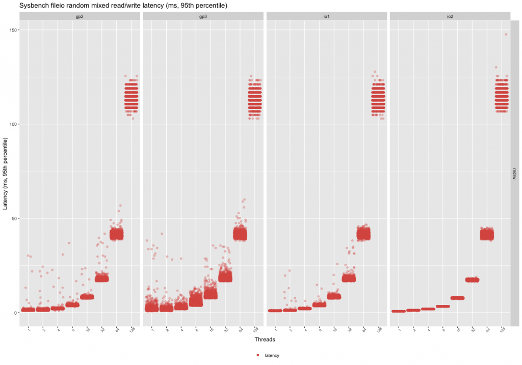
EBS storage type choices in AWS can be impacted by a lot of factors. As a consultant, I get a lot of questions about choosing the best storage type for a workload. Let me share a few examples. Is io2 better than gp2/3 if the configured iops are the same? What can I expect when upgrading gp2 to gp3?

In order to be able to answer questions like this, in this blog post, we will take a deeper look. We will compare storage devices that are “supposed to be the same”, in order to reveal the differences between these storage types. We will examine the following storage devices:

1 TB gp2 volume (has 3000 iops by definition)

1 TB gp3 volume, with the iops set to 3000

1 TB io1 volume, with the iops set to 3000

1 TB io2 volume, with the iops set to 3000

So, all the volumes are 1TB with 3000 iops, so in theory, they are the same. Also, in theory, theory and practice are the same, but in practice, they are different. Storage performance is more complex than just capacity and the number of iops, as we will see soon. Note that this test is very limited to draw conclusions like io1 is better than gp2 or anything like that in general. These devices have very different scalability characteristics (the io devices are scaling to 64k iops, while the maximum for the gp devices is 16k). Measuring the scalability of these devices and testing them in the long run and in different availability zones are out of scope for these tests. The reason I chose devices that have the same “specs” is to gain an understanding of the difference in their behavior. The tests were only run in a single availability zone (eu-west-1a).

For the tests, I used sysbench fileio, with the following prepare command.

sysbench --test=fileio \
--file-total-size=700G \
--threads=16 \
--file-num=64 \
--file-block-size=16384 \
prepare

The instances I used were r5.xlarge instances, which have up to 4750 Mbps bandwidth to EBS.

I used the following command to run the tests:

sysbench fileio \
--file-total-size=700G \
--time=1800 \
--max-requests=0 \
--threads=${th} \
--file-num=64 \
--file-io-mode=sync \
--file-test-mode=${test_mode} \
--file-extra-flags=direct \
--file-fsync-freq=0 \
--file-block-size=16384 \
--report-interval=1 \
run

In this command, the test mode can be rndwr (random writes only), rndrd (random reads only), and rndwr (random reads and writes mixed). The number of threads used were 1, 2, 4, 8, 16, 32, 64, and 128. All tests are using 16k io operations with direct io enabled (bypassing the filesystem cache), based on this, the peak theoretical throughput of the tests is 16k*3000 = 48 MB/s.

Random Writes

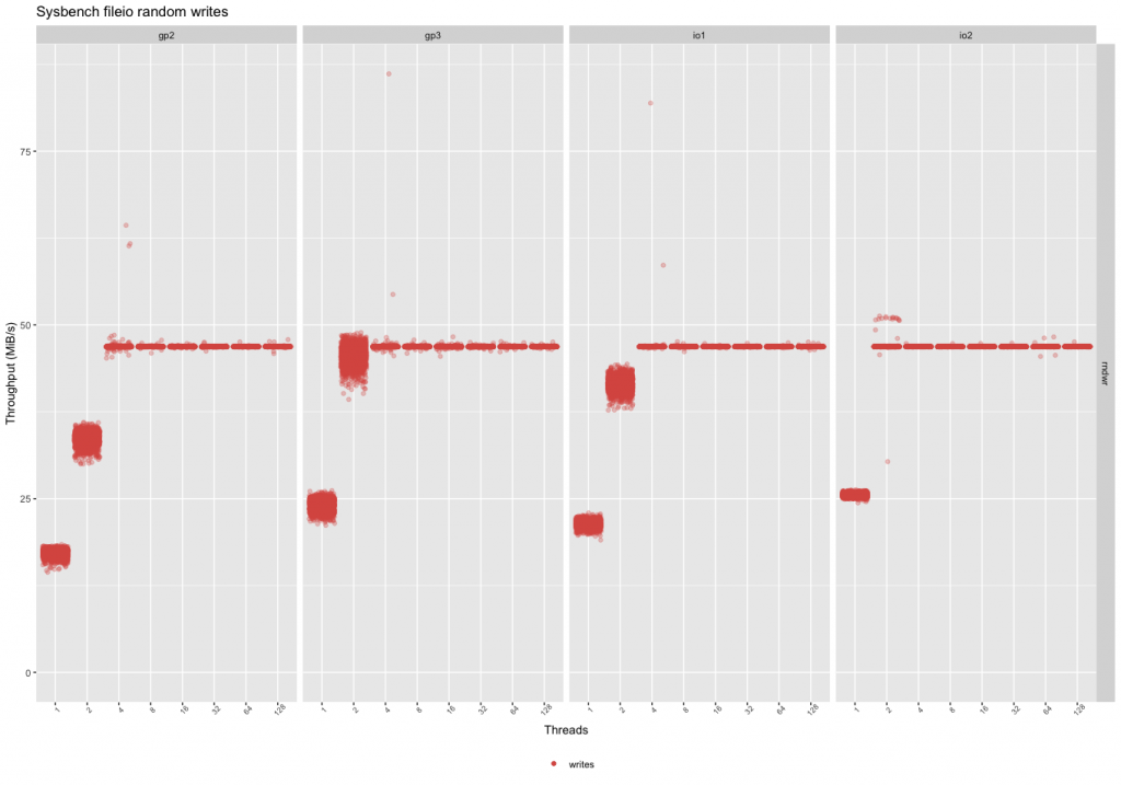
The gp2 and io1 devices reached the peak throughput for this benchmark with 4 threads and the gp3 reached it with 2 threads (but with a larger variance). The io2 device has more consistent performance overall. The peak throughput in these tests is the expected peak throughput (16k*3000 iops = 46.8MB/sec).

At a low thread count, gp3 has the highest variation in latency, gp2’s performance is more consistent. The latencies of io1 and io2 are more consistent, especially io2 at a higher thread count.

This means if the workload is mostly writes:

– Prefer gp3 over gp2 (better performance, less price).
– Prefer io2 if the price is worth the consistency in performance at lower thread counts.
– If the workload is multithreaded, and there are always more than 4 threads, prefer gp3 (in this case, the performance is the same, gp3 is the cheapest option).

Random Reads

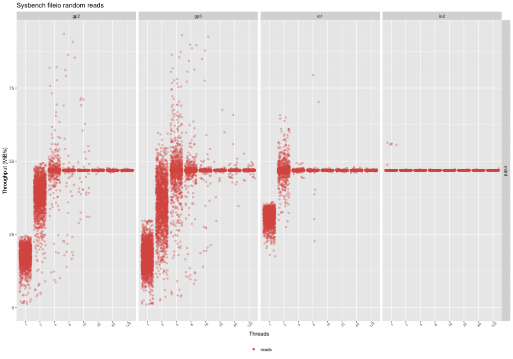
The random read throughput shows a much bigger difference than writes. First of all, the performance is more inconsistent in the case of gp2 and gp3, but gp2 seems to be slightly more consistent. The io2 device has the same consistent performance even with a single thread.

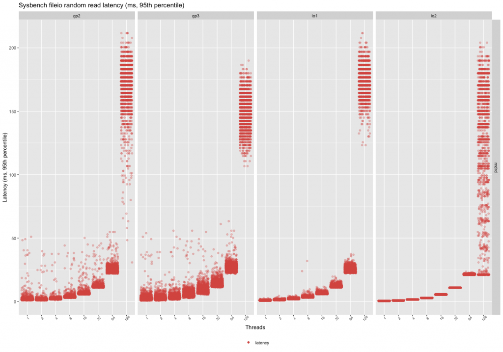
Similarly, there is a much bigger variance in latency in the case of low thread counts between the gp2 and the gp3. Even at 64 threads, the io2 device has very consistent latency characteristics.

This means if the workload is mostly reads:

– The gp2 volumes can give slightly better performance, but they are also slightly more expensive.
– Above 16 parallel threads, the devices are fairly similar, prefer gp3 because of the price.
– Prefer io2 if performance and latency are important with a low thread count (even over io1).

Random Mixed Reads/Writes

The mixed workload behavior is similar to the random read one, so the variance in the read performance will also show as a variance in the write performance. The more reads are added to the mix, the inconsistent the performance will become with the gp2/gp3 volumes. The io1 volume reaches peak throughput even with two threads, but with a high variance.

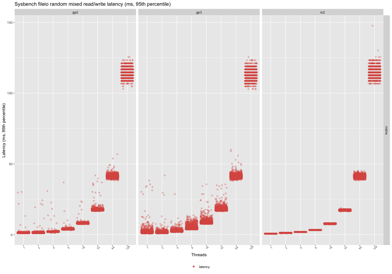
In the case of the mixed workload, the gp3 has the least consistent performance. This can come as an unpleasant surprise when the volumes are upgraded to gp3, and the workload has a low concurrency. This can be an issue for not loaded, but latency-sensitive applications. Otherwise, for choosing storage, the same advice applies to random reads.

Conclusion

The difference between these seemingly similar devices is greatest when a low number of threads are used against the device. If the io workload is parallel enough, the devices behave very similarly.

The raw data for these measurements are available on GitHub: https://github.com/pboros/aws_storage_blog.

As some of you likely know, I have a favorable view of ZFS and especially of MySQL on ZFS. As I published a few years ago, the argument for ZFS was less about performance than its useful features like data compression and snapshots. At the time, ZFS was significantly slower than xfs and ext4 except when the L2ARC was used.

Since then, however, ZFS on Linux has progressed a lot and I also learned how to better tune it. Also, I found out the sysbench benchmark I used at the time was not a fair choice since the dataset it generates compresses much less than a realistic one. For all these reasons, I believe that it is time to revisit the performance aspect of MySQL on ZFS.

ZFS Evolution

In 2018, I reported ZFS performance results based on version 0.6.5.6, the default version available in Ubuntu Xenial. The present post is using version 0.8.6-1 of ZFS, the default one available on Debian Buster. Between the two versions, there are in excess of 3600 commits adding a number of new features like support for trim operations and the addition of the efficient zstd compression algorithm.

ZFS 0.8.6-1 is not bleeding edge, there have been more than 1700 commits since and after 0.8.6, the ZFS release number jumped to 2.0. The big addition included in the 2.0 release is native encryption.

Benchmark Tools

The classic sysbench MySQL database benchmarks have a dataset containing mostly random data. Such datasets don’t compress much, less than most real-world datasets I worked with. The compressibility of the dataset is important since ZFS caches, the ARC and L2ARC, store compressed data. A better compression ratio essentially means more data is cached and fewer IO operations will be needed.

A well-known tool to benchmark a transactional workload is TPCC. Furthermore, the dataset created by TPCC compresses rather well making it more realistic in the context of this post. The sysbench TPCC implementation was used.

Test Environment

Since I am already familiar with AWS and Google cloud, I decided to try Azure for this project. I launched these two virtual machines:

tpcc:

• benchmark host
• Standard D2ds_v4 instance
• 2 vCpu, 8GB of Ram and 75 GB of temporary storage
• Debian Buster

db:

• Database host
• Standard E4-2ds-v4 instance
• 2 vCpu, 32GB of Ram and 150GB of temporary storage
• 256GB SSD Premium (SSD Premium LRS P15 – 1100 IOPS (3500 burst), 125 MB/s)
• Debian Buster
• Percona server 8.0.22-13

Configuration

By default and unless specified, the ZFS filesystems are created with:

zpool create bench /dev/sdc
zfs set compression=lz4 atime=off logbias=throughput bench
zfs create -o mountpoint=/var/lib/mysql/data -o recordsize=16k \
           -o primarycache=metadata bench/data
zfs create -o mountpoint=/var/lib/mysql/log bench/log

There are two ZFS filesystems. bench/data is optimized for the InnoDB dataset while bench/log is tuned for the InnoDB log files. Both are compressed using lz4 and the logbias parameter is set to throughput which changes the way the ZIL is used. With ext4, the noatime option is used.

ZFS has also a number of kernel parameters, the ones set to non-default values are:

zfs_arc_max=2147483648
zfs_async_block_max_blocks=5000
zfs_delete_blocks=1000

Essentially, the above settings limit the ARC size to 2GB and they throttle down the aggressiveness of ZFS for deletes. Finally, the database configuration is slightly different between ZFS and ext4. There is a common section:

[mysqld]
pid-file = /var/run/mysqld/mysqld.pid
socket = /var/run/mysqld/mysqld.sock
log-error = /var/log/mysql/error.log
skip-log-bin
datadir = /var/lib/mysql/data
innodb_buffer_pool_size = 26G
innodb_flush_log_at_trx_commit = 1 # TPCC reqs.
innodb_log_file_size = 1G
innodb_log_group_home_dir = /var/lib/mysql/log
innodb_flush_neighbors = 0
innodb_fast_shutdown = 2

and when ext4 is used:

innodb_flush_method = O_DIRECT

and when ZFS is used:

innodb_flush_method = fsync
innodb_doublewrite = 0 # ZFS is transactional
innodb_use_native_aio = 0
innodb_read_io_threads = 10
innodb_write_io_threads = 10

ZFS doesn’t support O_DIRECT but it is ignored with a message in the error log. I chose to explicitly set the flush method to fsync. The doublewrite buffer is not needed with ZFS and I was under the impression that the Linux native asynchronous IO implementation was not well supported by ZFS so I disabled it and increased the number of IO threads. We’ll revisit the asynchronous IO question in a future post.

Dataset

I use the following command to create the dataset:

./tpcc.lua --mysql-host=10.3.0.6 --mysql-user=tpcc --mysql-password=tpcc --mysql-db=tpcc \
--threads=8 --tables=10 --scale=200 --db-driver=mysql prepare

The resulting dataset has a size of approximately 200GB. The dataset is much larger than the buffer pool so the database performance is essentially IO-bound.

Test Procedure

The execution of every benchmark was scripted and followed these steps:

1. Stop MySQL
2. Remove all datafiles
3. Adjust the filesystem
4. Copy the dataset
5. Adjust the MySQL configuration
6. Start MySQL
7. Record the configuration
8. Run the benchmark

Results

For the benchmark, I used the following invocation:

./tpcc.lua --mysql-host=10.3.0.6 --mysql-user=tpcc --mysql-password=tpcc --mysql-db=tpcc \
--threads=16 --time=7200 --report-interval=10 --tables=10 --scale=200 --db-driver=mysql ru

The TPCC benchmark uses 16 threads for a duration of 2 hours. The duration is sufficiently long to allow for a steady state and to exhaust the storage burst capacity. Sysbench returns the total number of TPCC transactions per second every 10s. This number includes not only the New Order transactions but also the other transaction types like payment, order status, etc. Be aware of that if you want to compare these results with other TPCC benchmarks.

In those conditions, the figure below presents the rates of TPCC transactions over time for ext4 and ZFS.

During the initial 15 minutes, the buffer pool warms up but at some point, the workload shifts between an IO read bound to an IO write and CPU bound. Then, at around 3000s the SSD Premium burst capacity is exhausted and the workload is only IO-bound. I have been a bit surprised by the results, enough to rerun the benchmarks to make sure. The results for both ext4 and ZFS are qualitatively similar. Any difference is within the margin of error. That essentially means if you configure ZFS properly, it can be as IO efficient as ext4.

What is interesting is the amount of storage used. While the dataset on ext4 consumed 191GB, the lz4 compression of ZFS yielded a dataset of only 69GB. That’s a huge difference, a factor of 2.8, which could save a decent amount of money over time for large datasets.

Conclusion

It appears that it was indeed a good time to revisit the performance of MySQL with ZFS. In a fairly realistic use case, ZFS is on par with ext4 regarding performance while still providing the extra benefits of data compression, snapshots, etc. In a future post, I’ll examine the use of cloud ephemeral storage with ZFS and see how this can further improve performance.

It’s your busiest day of the year and the website has crawled to a halt and finally crashed… and it was all because you did not understand how MongoDB uses memory and left your system open to cluster instability, poor performance, and unpredictable behavior. Understanding how MongoDB uses memory and planning for its use can save you a lot of headaches, tears, and grief. Over the last 5 years, I have too often been called in to fix what are easily avoided problems. Let me share with you how MongoDB uses Memory, and how to avoid potentially disastrous mistakes when using MongoDB.

In most databases, more data cached in RAM is better. Same in MongoDB. However, cache competes with other memory-intensive processes as well as the kernel ones.

To speed up performance many people simply allocate the resources to the most visible issue. In the case of MongoDB however, sometimes allocating more memory actually hurts performance. How is this possible? The short answer is MongoDB relies on both its internal memory caches as well as the operating system’s cache. The OS cache generally is seen as “Unallocated” by sysadmins, dba’s, and devs. This means they steal memory from the OS and allocate it internally to MongoDB. Why is this potentially a bad thing? Let me explain.

How MongoDB Uses the Memory for Caching Data

Anytime you run a query some pages are copied from the files into an internal memory cache of the mongod process for future reuse. A part of your data and indexes can be cached and retrieved really very fast when needed. This is what the WiredTiger Cache (WTC) does. The goal of the WTC is to store the most frequently and recently used pages in order to provide the fastest access to your data. That’s awesome for improving the performance of the database.

By default, a mongod process uses up to 50% of the available RAM for that cache. Eventually, you can change the size of the WTC using the  storage.wiredTiger.engineConfig.cacheSizeGB configuration variable.

Remember that the data is compressed on disk files while the cache stores instead uncompressed pages.

When the WTC gets close to full, more evictions can happen. Evictions happen when the requested pages are not in the cache and mongod has to drop out existing pages in order to make room and read the incoming pages from the file system. The eviction walk algorithm does a few other things (LRU page list sorting and WT page reconciliation) as well as marking the least recently used pages as available for reuse, and altogether this can cause at some point slowness because of a more intensive IO.

Based on how the WTC works, someone could think it’s a good idea to assign even 80%/90% of the memory to it (if you are familiar with MySQL, it’s the same you do when configuring the Buffer Pool for InnoDB). Most of the time this is a mistake and to understand why let’s see now another way mongod uses the memory.

How MongoDB Uses the Memory for File Buffering

Sudden topic change: we’re going to talk about OS instead for a bit. The OS also caches into the memory normal filesystem disk blocks in order to speed up their retrieval if they are requested multiple times. This feature is provided by the system regardless of which application is using it, and it’s really beneficial when an application needs frequent access to the disk. When the IO operation is triggered, the data can be returned by reading the blocks from the memory instead of accessing the disk for real. Then the request will be served faster. This kind of memory managed by the OS is called cached, as you see in /proc/meminfo. We can also call it “File Buffering”.

# cat /proc/meminfo 
MemTotal:        1882064 kB
MemFree:         1376380 kB
MemAvailable:    1535676 kB
Buffers:            2088 kB
Cached:           292324 kB
SwapCached:            0 kB
Active:           152944 kB
Inactive:         252628 kB
Active(anon):     111328 kB
Inactive(anon):    16508 kB
Active(file):      41616 kB
Inactive(file):   236120 kB
Unevictable:           0 kB
Mlocked:               0 kB
SwapTotal:       2097148 kB
SwapFree:        2097148 kB
Dirty:                40 kB
Writeback:             0 kB
AnonPages:        111180 kB
Mapped:            56396 kB
...
[truncated]

Keep in mind that MongoDB relies entirely on the Operating System for file buffering.

On a dedicated server, where running a single mongod process, as long as you use the database more disk blocks will be stored into the memory. In the end, almost all the “cached” + “buffer” fields in the memory stat output shown above will be used exclusively for the disk blocks requested by mongod.

An important thing is that the cached memory saves the disk blocks exactly as they are. Since the disk blocks are compressed into the WT files, also the blocks into the memory are compressed. Because of the compression, you can store really a lot of your MongoDB data and indexes.

Let’s suppose you have a 4x compression ratio, in a 10GB memory file buffer (cached memory) you can store up to 40GB of real data. That’s a lot more, for free.

Putting Things Together

The following picture gives you a rough overview of memory usage.

Suppose we have a dedicated 64GB RAM machine and a 120GB dataset. Because of compression, the database uses around 30GB of storage, assuming a 4x compression ratio, which is quite common.

Without changing anything on the configuration, then around 32GB will be used by the WTC for saving 32GB of uncompressed data. The remaining memory will be used in part by the OS and other applications and let’s say it is 4GB. The remaining RAM is 28GB and it will be mainly used for file buffering. In that 28 GB, we can store almost the entire compressed database. The overall performance of MongoDB will be great because most of the time it won’t read from disk. Only 2GB of the compressed file data are not stored on File Buffering. Or 8GB of the uncompressed 120GB as another way to look at it. So, when there’s an access on a page not amongst the 32GB in the  WTC at that moment the IO will read a disk block most probably from the File Buffer instead of doing real disk access. At least 10x better latency, maybe 100x. That’s awesome.

Multiple mongod on the Same Machine is Bad

As I mentioned, people hate to see that (apparently) unallocated memory on their systems.  Not everyone with that misconception increases the WTC, sometimes they view this as an opportunity to add other mongods on the same box, to use that unused memory.

The multiple mongod processes would like all their disk file content to be cached in memory by the OS too. You can limit the size of the WTC, but you cannot affect the requests to the disk and the file buffering usage. This causes less memory used for the file buffering for any mongod process triggering more real disk IO. In addition, the processes will compete for accessing other resources, like the CPU.

Another problem is that multiple mongod processes make troubleshooting more complicated. It won’t be so simple to identify the root cause of any issue. Which mongod is using more memory for file buffering? Is the other mongod’s slowness affecting the performance of my mongod?

Troubleshooting can be addressed easier on a dedicated machine when running a single mongod.

If one of the mongods gets crazy and uses more CPU time and memory, then all the mongods on the machine will slow down because of fewer resources available in the system.

In the end, never deploy more than one mongod on the same machine. Eventually, you may consider Docker containers. Running mongod in a container you can limit the amount of memory it can use. In such a case do your calculations for how much memory you need in total for the server and how much memory reserve for any container to get the best possible performance for mongod.

It is Not Recommended to Have a Very Large WTC

Increasing the WTC significantly, more than the 50% default, is also a bad habit.

With a larger cache, you can store more uncompressed data but at the same time, you leave a little memory for file buffering. More queries can benefit from the larger WTC but when having evictions mongod could trigger a lot of real disk accesses slowing down the database.

For this reason, in most cases, it is not recommended to increase the WTC higher than the default 50%. The goal is to save enough space for buffering disk blocks into the memory. This can help you to get a very good and more stable performance.

Conclusion

When you think about mongod, you have to consider it as the only process running in the universe. It tries to use as much memory as it can. But there are two caches – the WT cache (uncompressed documents) and the file buffer (of WiredTiger’s compressed files), and performance will be hurt if you starve one for the other.

Never deploy multiple mongods into the same box or at least consider containers. For the WTC, also remember that most of the time the default size (up to 50% of the RAM) works well.